Take-home Exercise 3: Predicting HDB Public Housing Resale Pricies using Geographically Weighted Methods

1 Overview

1.1 Setting the Scene

Housing is an essential component of household wealth worldwide. Buying a housing has always been a major investment for most people. The price of housing is affected by many factors. Some of them are global in nature such as the general economy of a country or inflation rate. Others can be more specific to the properties themselves. These factors can be further divided to structural and locational factors. Structural factors are variables related to the property themselves such as the size, fitting, and tenure of the property. Locational factors are variables related to the neighbourhood of the properties such as proximity to childcare centre, public transport service and shopping centre.

Conventional, housing resale prices predictive models were built by using Ordinary Least Square (OLS) method. However, this method failed to take into consideration that spatial autocorrelation and spatial heterogeneity exist in geographic data sets such as housing transactions. With the existence of spatial autocorrelation, the OLS estimation of predictive housing resale pricing models could lead to biased, inconsistent, or inefficient results (Anselin 1998). In view of this limitation, Geographical Weighted Models were introduced for calibrating predictive model for housing resale prices.

1.2 The Task

In this take-home exercise, you are tasked to predict HDB resale prices at the sub-market level (i.e. HDB 3-room, HDB 4-room and HDB 5-room) for the month of January and February 2023 in Singapore. The predictive models must be built by using by using conventional OLS method and GWR methods. You are also required to compare the performance of the conventional OLS method versus the geographical weighted methods.

1.3 The Data

For the purpose of this take-home exercise, HDB Resale Flat Prices provided by Data.gov.sg should be used as the core data set. The study should focus on either three-room, four-room or five-room flat and transaction period should be from 1st January 2021 to 31st December 2022. The test data should be January and February 2023 resale prices.

Aspatial Data Set	Source
HDB Resale Data	Data.gov.sg

Geospatial Data Set	Source
Master Plan 2019 Sub-Zone Boundary	Prof. Kam
Hawker Centres	OneMap
Childcare Centres	OneMap
Kindergartens	OneMap
NParks Parks and Nature Reserves	OneMap
Shopping Malls	Wikipedia; GitHub - ValaryLim
Supermarket	Data.gov.sg
Eldercare	Data.gov.sg
MRT Stations	LTA DataMall
Bus Stops	LTA DataMall

1.4 Acknowledgement

Name	Source
Prof. Kam	Hands-On Ex 8; In-Class Ex 9
Megan Sim	Take-Home Ex 3
Nor Aisyah Binte Ajit	Take-Home Ex 3

2 Getting Started

2.1 Import Packages

packages <- c('sf', 'tidyverse', 'tmap', 'httr', 'jsonlite', 'rvest', 
              'sp', 'ggpubr', 'corrplot', 'broom',  'olsrr', 'spdep', 
              'GWmodel', 'devtools', 'rgeos', 'lwgeom', 'maptools', 'matrixStats',
              'units', 'gtsummary', 'Metrics', 'rsample', 'SpatialML')

for(p in packages){
  if(!require(p, character.only = T)){
    install.packages(p, repos = "http://cran.us.r-project.org")
  }
  library(p, character.only = T)
}

2.2 Importing Aspatial Data

resale <- read_csv("data/aspatial/resale-flat-prices-based-on-registration-date-from-jan-2017-onwards.csv")

head(resale)

# A tibble: 6 × 11
  month   town     flat_…¹ block stree…² store…³ floor…⁴ flat_…⁵ lease…⁶ remai…⁷
  <chr>   <chr>    <chr>   <chr> <chr>   <chr>     <dbl> <chr>     <dbl> <chr>  
1 2017-01 ANG MO … 2 ROOM  406   ANG MO… 10 TO …      44 Improv…    1979 61 yea…
2 2017-01 ANG MO … 3 ROOM  108   ANG MO… 01 TO …      67 New Ge…    1978 60 yea…
3 2017-01 ANG MO … 3 ROOM  602   ANG MO… 01 TO …      67 New Ge…    1980 62 yea…
4 2017-01 ANG MO … 3 ROOM  465   ANG MO… 04 TO …      68 New Ge…    1980 62 yea…
5 2017-01 ANG MO … 3 ROOM  601   ANG MO… 01 TO …      67 New Ge…    1980 62 yea…
6 2017-01 ANG MO … 3 ROOM  150   ANG MO… 01 TO …      68 New Ge…    1981 63 yea…
# … with 1 more variable: resale_price <dbl>, and abbreviated variable names
#   ¹​flat_type, ²​street_name, ³​storey_range, ⁴​floor_area_sqm, ⁵​flat_model,
#   ⁶​lease_commence_date, ⁷​remaining_lease

2.2.1 Filter Resale Data

Resale Data filter includes both training data and test data set

resale_filter <- filter(resale, flat_type == "4 ROOM") %>%
  filter(month >= "2021-01" & month <= "2023-02")

2.2.1.1 Glimpse Filtered Resale Data

glimpse(resale_filter)

Rows: 25,502
Columns: 11
$ month               <chr> "2021-01", "2021-01", "2021-01", "2021-01", "2021-…
$ town                <chr> "ANG MO KIO", "ANG MO KIO", "ANG MO KIO", "ANG MO …
$ flat_type           <chr> "4 ROOM", "4 ROOM", "4 ROOM", "4 ROOM", "4 ROOM", …
$ block               <chr> "547", "414", "509", "467", "571", "134", "204", "…
$ street_name         <chr> "ANG MO KIO AVE 10", "ANG MO KIO AVE 10", "ANG MO …
$ storey_range        <chr> "04 TO 06", "01 TO 03", "01 TO 03", "07 TO 09", "0…
$ floor_area_sqm      <dbl> 92, 92, 91, 92, 92, 98, 92, 92, 92, 92, 92, 109, 9…
$ flat_model          <chr> "New Generation", "New Generation", "New Generatio…
$ lease_commence_date <dbl> 1981, 1979, 1980, 1979, 1979, 1978, 1977, 1978, 19…
$ remaining_lease     <chr> "59 years", "57 years 09 months", "58 years 06 mon…
$ resale_price        <dbl> 370000, 375000, 380000, 385000, 410000, 410000, 41…

2.2.1.2 Check for Correct Time Period

unique(resale_filter$month)

 [1] "2021-01" "2021-02" "2021-03" "2021-04" "2021-05" "2021-06" "2021-07"
 [8] "2021-08" "2021-09" "2021-10" "2021-11" "2021-12" "2022-01" "2022-02"
[15] "2022-03" "2022-04" "2022-05" "2022-06" "2022-07" "2022-08" "2022-09"
[22] "2022-10" "2022-11" "2022-12" "2023-01" "2023-02"

2.2.1.3 Check for Correct Flat Type

unique(resale_filter$flat_type)

[1] "4 ROOM"

2.2.2 Transform Resale Data

2.2.2.1 Adding New Columns

resale_transform <- resale_filter %>%
  mutate(resale_filter, address = paste(block,street_name)) %>%
  mutate(resale_filter, remaining_lease_yr = as.integer(str_sub(remaining_lease, 0, 2))) %>%
  mutate(resale_filter, remaining_lease_mth = as.integer(str_sub(remaining_lease, 9, 11)))

2.2.2.2 Replace NA Values in “remaining_lease_mth”

resale_transform$remaining_lease_mth[is.na(resale_transform$remaining_lease_mth)] <- 0

2.2.2.3 Convert “remaining_lease_yr” to Months

resale_transform$remaining_lease_yr <- resale_transform$remaining_lease_yr * 12
resale_transform <- resale_transform %>%
  mutate(resale_transform, remaining_lease_mths = rowSums(resale_transform[, c("remaining_lease_yr", "remaining_lease_mth")])) %>%
  select(month, town, address, block, street_name, flat_type, storey_range, floor_area_sqm, flat_model, 
         lease_commence_date, remaining_lease_mths, resale_price)

2.2.3 Getting Unique Addresses

address <- sort(unique(resale_transform$address))

head(address)

[1] "1 CHAI CHEE RD"    "1 PINE CL"         "1 ST. GEORGE'S RD"
[4] "1 TECK WHYE AVE"   "1 TOH YI DR"       "10 CHAI CHEE RD"  

2.2.4 Getting LAT & LONG from OneMap.sg API

get_coords <- function(add_list){
  
  # Create a data frame to store all retrieved coordinates
  postal_coords <- data.frame()
    
  for (i in add_list){
    #print(i)

    r <- GET('https://developers.onemap.sg/commonapi/search?',
           query=list(searchVal=i,
                     returnGeom='Y',
                     getAddrDetails='Y'))
    data <- fromJSON(rawToChar(r$content))
    found <- data$found
    res <- data$results
    
    # Create a new data frame for each address
    new_row <- data.frame()
    
    # If single result, append 
    if (found == 1){
      postal <- res$POSTAL 
      lat <- res$LATITUDE
      lng <- res$LONGITUDE
      new_row <- data.frame(address= i, postal = postal, latitude = lat, longitude = lng)
    }
    
    # If multiple results, drop NIL and append top 1
    else if (found > 1){
      # Remove those with NIL as postal
      res_sub <- res[res$POSTAL != "NIL", ]
      
      # Set as NA first if no Postal
      if (nrow(res_sub) == 0) {
          new_row <- data.frame(address= i, postal = NA, latitude = NA, longitude = NA)
      }
      
      else{
        top1 <- head(res_sub, n = 1)
        postal <- top1$POSTAL 
        lat <- top1$LATITUDE
        lng <- top1$LONGITUDE
        new_row <- data.frame(address= i, postal = postal, latitude = lat, longitude = lng)
      }
    }

    else {
      new_row <- data.frame(address= i, postal = NA, latitude = NA, longitude = NA)
    }
    
    # Add the row
    postal_coords <- rbind(postal_coords, new_row)
  }
  return(postal_coords)
}

2.2.4.1 Calling Function

latlong <- get_coords(address)

2.2.4.2 Check for Missing Value

latlong[(is.na(latlong))]

character(0)

2.2.5 Combine Resale and LAT & LONG

resale_latlong <- left_join(resale_transform, latlong, by = c('address' = 'address'))

head(resale_latlong)

# A tibble: 6 × 15
  month   town     address block stree…¹ flat_…² store…³ floor…⁴ flat_…⁵ lease…⁶
  <chr>   <chr>    <chr>   <chr> <chr>   <chr>   <chr>     <dbl> <chr>     <dbl>
1 2021-01 ANG MO … 547 AN… 547   ANG MO… 4 ROOM  04 TO …      92 New Ge…    1981
2 2021-01 ANG MO … 414 AN… 414   ANG MO… 4 ROOM  01 TO …      92 New Ge…    1979
3 2021-01 ANG MO … 509 AN… 509   ANG MO… 4 ROOM  01 TO …      91 New Ge…    1980
4 2021-01 ANG MO … 467 AN… 467   ANG MO… 4 ROOM  07 TO …      92 New Ge…    1979
5 2021-01 ANG MO … 571 AN… 571   ANG MO… 4 ROOM  07 TO …      92 New Ge…    1979
6 2021-01 ANG MO … 134 AN… 134   ANG MO… 4 ROOM  07 TO …      98 New Ge…    1978
# … with 5 more variables: remaining_lease_mths <dbl>, resale_price <dbl>,
#   postal <chr>, latitude <chr>, longitude <chr>, and abbreviated variable
#   names ¹​street_name, ²​flat_type, ³​storey_range, ⁴​floor_area_sqm,
#   ⁵​flat_model, ⁶​lease_commence_date

2.2.6 Check for NA

resale_latlong[(is.na(resale_latlong))]

<unspecified> [0]

2.2.7 Write File to rds

resale_latlong.rds <- write_rds(resale_latlong, "data/model/resale_latlong.rds")

2.2.8 Read resale_rds File

resale_main <- read_rds("data/model/resale_latlong.rds")

head(resale_main)

# A tibble: 6 × 15
  month   town     address block stree…¹ flat_…² store…³ floor…⁴ flat_…⁵ lease…⁶
  <chr>   <chr>    <chr>   <chr> <chr>   <chr>   <chr>     <dbl> <chr>     <dbl>
1 2021-01 ANG MO … 547 AN… 547   ANG MO… 4 ROOM  04 TO …      92 New Ge…    1981
2 2021-01 ANG MO … 414 AN… 414   ANG MO… 4 ROOM  01 TO …      92 New Ge…    1979
3 2021-01 ANG MO … 509 AN… 509   ANG MO… 4 ROOM  01 TO …      91 New Ge…    1980
4 2021-01 ANG MO … 467 AN… 467   ANG MO… 4 ROOM  07 TO …      92 New Ge…    1979
5 2021-01 ANG MO … 571 AN… 571   ANG MO… 4 ROOM  07 TO …      92 New Ge…    1979
6 2021-01 ANG MO … 134 AN… 134   ANG MO… 4 ROOM  07 TO …      98 New Ge…    1978
# … with 5 more variables: remaining_lease_mths <dbl>, resale_price <dbl>,
#   postal <chr>, latitude <chr>, longitude <chr>, and abbreviated variable
#   names ¹​street_name, ²​flat_type, ³​storey_range, ⁴​floor_area_sqm,
#   ⁵​flat_model, ⁶​lease_commence_date

2.2.9 Transform to sf and Assign CRS

resale_main_sf <- st_as_sf(resale_main,
                    coords = c("longitude", 
                               "latitude"),
                    crs=4326) %>%
  st_transform(crs = 3414)

st_crs(resale_main_sf)

Coordinate Reference System:
  User input: EPSG:3414 
  wkt:
PROJCRS["SVY21 / Singapore TM",
    BASEGEOGCRS["SVY21",
        DATUM["SVY21",
            ELLIPSOID["WGS 84",6378137,298.257223563,
                LENGTHUNIT["metre",1]]],
        PRIMEM["Greenwich",0,
            ANGLEUNIT["degree",0.0174532925199433]],
        ID["EPSG",4757]],
    CONVERSION["Singapore Transverse Mercator",
        METHOD["Transverse Mercator",
            ID["EPSG",9807]],
        PARAMETER["Latitude of natural origin",1.36666666666667,
            ANGLEUNIT["degree",0.0174532925199433],
            ID["EPSG",8801]],
        PARAMETER["Longitude of natural origin",103.833333333333,
            ANGLEUNIT["degree",0.0174532925199433],
            ID["EPSG",8802]],
        PARAMETER["Scale factor at natural origin",1,
            SCALEUNIT["unity",1],
            ID["EPSG",8805]],
        PARAMETER["False easting",28001.642,
            LENGTHUNIT["metre",1],
            ID["EPSG",8806]],
        PARAMETER["False northing",38744.572,
            LENGTHUNIT["metre",1],
            ID["EPSG",8807]]],
    CS[Cartesian,2],
        AXIS["northing (N)",north,
            ORDER[1],
            LENGTHUNIT["metre",1]],
        AXIS["easting (E)",east,
            ORDER[2],
            LENGTHUNIT["metre",1]],
    USAGE[
        SCOPE["Cadastre, engineering survey, topographic mapping."],
        AREA["Singapore - onshore and offshore."],
        BBOX[1.13,103.59,1.47,104.07]],
    ID["EPSG",3414]]

2.2.10 Check for Invalid Geometries

length(which(st_is_valid(resale_main_sf) == FALSE))

[1] 0

2.3 Importing Geospatial Data

Importing Master Plan 2019 Subzone

mpsz <- st_read(dsn = "data/geospatial", layer = "MPSZ-2019")

Reading layer `MPSZ-2019' from data source 
  `C:\Users\la935\Desktop\IS415 - GAA\IS415 - GAA (New)\Take-Home_Ex\Take-Home_Ex03\data\geospatial' 
  using driver `ESRI Shapefile'
Simple feature collection with 332 features and 6 fields
Geometry type: MULTIPOLYGON
Dimension:     XY
Bounding box:  xmin: 103.6057 ymin: 1.158699 xmax: 104.0885 ymax: 1.470775
Geodetic CRS:  WGS 84

Check for Invalid Geometry

length(which(st_is_valid(mpsz) == FALSE))

[1] 6

Make Geometry Valid and Check for Invalid Geometry Again

mpsz <- st_make_valid(mpsz)
length(which(st_is_valid(mpsz) == FALSE))

[1] 0

Assign ESPG Code

mpsz <- st_transform(mpsz, 3414)
st_crs(mpsz)

Coordinate Reference System:
  User input: EPSG:3414 
  wkt:
PROJCRS["SVY21 / Singapore TM",
    BASEGEOGCRS["SVY21",
        DATUM["SVY21",
            ELLIPSOID["WGS 84",6378137,298.257223563,
                LENGTHUNIT["metre",1]]],
        PRIMEM["Greenwich",0,
            ANGLEUNIT["degree",0.0174532925199433]],
        ID["EPSG",4757]],
    CONVERSION["Singapore Transverse Mercator",
        METHOD["Transverse Mercator",
            ID["EPSG",9807]],
        PARAMETER["Latitude of natural origin",1.36666666666667,
            ANGLEUNIT["degree",0.0174532925199433],
            ID["EPSG",8801]],
        PARAMETER["Longitude of natural origin",103.833333333333,
            ANGLEUNIT["degree",0.0174532925199433],
            ID["EPSG",8802]],
        PARAMETER["Scale factor at natural origin",1,
            SCALEUNIT["unity",1],
            ID["EPSG",8805]],
        PARAMETER["False easting",28001.642,
            LENGTHUNIT["metre",1],
            ID["EPSG",8806]],
        PARAMETER["False northing",38744.572,
            LENGTHUNIT["metre",1],
            ID["EPSG",8807]]],
    CS[Cartesian,2],
        AXIS["northing (N)",north,
            ORDER[1],
            LENGTHUNIT["metre",1]],
        AXIS["easting (E)",east,
            ORDER[2],
            LENGTHUNIT["metre",1]],
    USAGE[
        SCOPE["Cadastre, engineering survey, topographic mapping."],
        AREA["Singapore - onshore and offshore."],
        BBOX[1.13,103.59,1.47,104.07]],
    ID["EPSG",3414]]

2.3.1 Data With LAT & LONG

2.3.1.1 Elderly Care

elder_sf <- st_read(dsn = "data/geospatial", layer = "ELDERCARE")

Reading layer `ELDERCARE' from data source 
  `C:\Users\la935\Desktop\IS415 - GAA\IS415 - GAA (New)\Take-Home_Ex\Take-Home_Ex03\data\geospatial' 
  using driver `ESRI Shapefile'
Simple feature collection with 133 features and 18 fields
Geometry type: POINT
Dimension:     XY
Bounding box:  xmin: 14481.92 ymin: 28218.43 xmax: 41665.14 ymax: 46804.9
Projected CRS: SVY21

# Assign EPSG Code
elder_sf <- st_transform(elder_sf, 3414)

2.3.1.2 Bus Stops

BusStop_sf <- st_read(dsn = "data/geospatial", layer = "BusStop")

Reading layer `BusStop' from data source 
  `C:\Users\la935\Desktop\IS415 - GAA\IS415 - GAA (New)\Take-Home_Ex\Take-Home_Ex03\data\geospatial' 
  using driver `ESRI Shapefile'
Simple feature collection with 5159 features and 3 fields
Geometry type: POINT
Dimension:     XY
Bounding box:  xmin: 3970.122 ymin: 26482.1 xmax: 48284.56 ymax: 52983.82
Projected CRS: SVY21

# Assign EPSG Code
BusStop_sf <- st_transform(BusStop_sf, 3414)

2.3.1.3 MRT Stations

mrt <- read.csv("data/geospatial/mrtsg.csv")

mrt_sf <- st_as_sf(mrt,
                   coords = c("Longitude",
                              "Latitude"),
                              crs = 4326) %>%
  st_transform(crs = 3414)

2.3.1.4 Childcare Center

childcare_sf <- st_read(dsn = "data/geospatial", layer = "CHILDCARE")

Reading layer `CHILDCARE' from data source 
  `C:\Users\la935\Desktop\IS415 - GAA\IS415 - GAA (New)\Take-Home_Ex\Take-Home_Ex03\data\geospatial' 
  using driver `ESRI Shapefile'
Simple feature collection with 1545 features and 15 fields
Geometry type: POINT
Dimension:     XY
Bounding box:  xmin: 11203.01 ymin: 25667.6 xmax: 45404.24 ymax: 49300.88
Projected CRS: WGS_1984_Transverse_Mercator

# Assign EPSG Code
childcare_sf <- st_transform(childcare_sf, 3414)

2.3.1.5 Kindergarten

kindergarten_sf <- st_read(dsn = "data/geospatial", layer = "KINDERGARTENS")

Reading layer `KINDERGARTENS' from data source 
  `C:\Users\la935\Desktop\IS415 - GAA\IS415 - GAA (New)\Take-Home_Ex\Take-Home_Ex03\data\geospatial' 
  using driver `ESRI Shapefile'
Simple feature collection with 448 features and 15 fields
Geometry type: POINT
Dimension:     XY
Bounding box:  xmin: 11909.7 ymin: 25596.33 xmax: 43395.47 ymax: 48562.06
Projected CRS: SVY21

# Assign EPSG Code
kindergarten_sf <- st_transform(kindergarten_sf, 3414)

2.3.1.6 Parks

parks_sf <- st_read(dsn = "data/geospatial", layer = "NATIONALPARKS")

Reading layer `NATIONALPARKS' from data source 
  `C:\Users\la935\Desktop\IS415 - GAA\IS415 - GAA (New)\Take-Home_Ex\Take-Home_Ex03\data\geospatial' 
  using driver `ESRI Shapefile'
Simple feature collection with 352 features and 15 fields
Geometry type: POINT
Dimension:     XY
Bounding box:  xmin: 12373.11 ymin: 21869.93 xmax: 46735.95 ymax: 49231.09
Projected CRS: SVY21

# Assign EPSG Code
parks_sf <- st_transform(parks_sf, 3414)

2.3.1.6 Hawker Centre

hawker_sf <- st_read(dsn = "data/geospatial", layer = "HAWKERCENTRE")

Reading layer `HAWKERCENTRE' from data source 
  `C:\Users\la935\Desktop\IS415 - GAA\IS415 - GAA (New)\Take-Home_Ex\Take-Home_Ex03\data\geospatial' 
  using driver `ESRI Shapefile'
Simple feature collection with 125 features and 21 fields
Geometry type: POINT
Dimension:     XY
Bounding box:  xmin: 12874.19 ymin: 28355.97 xmax: 45241.4 ymax: 47872.53
Projected CRS: SVY21

# Assign EPSG Code
hawker_sf <- st_transform(hawker_sf, 3414)

2.3.1.7 Supermarkets

supermarket_sf <- st_read(dsn = "data/geospatial", layer = "SUPERMARKETS")

Reading layer `SUPERMARKETS' from data source 
  `C:\Users\la935\Desktop\IS415 - GAA\IS415 - GAA (New)\Take-Home_Ex\Take-Home_Ex03\data\geospatial' 
  using driver `ESRI Shapefile'
Simple feature collection with 526 features and 8 fields
Geometry type: POINT
Dimension:     XY
Bounding box:  xmin: 4901.188 ymin: 25529.08 xmax: 46948.22 ymax: 49233.6
Projected CRS: SVY21

# Assign EPSG Code
supermarket_sf <- st_transform(supermarket_sf, 3414)

2.3.2 Data Without LAT & LONG

2.3.2.1 CBD (Downtown Core, Singapore)

# Storing LAT & LONG for CBD as Dataframe
name <- c('CBD')
latitude = c(1.287953)
longitude = c(103.851784)
cbd <- data.frame(name, latitude, longitude)

# Convert to sf and Assign EPSG
cbd_sf <- st_as_sf(cbd,
                   coords = c("longitude",
                              "latitude"),
                   crs = 4326) %>%
  st_transform(crs = 3414)

st_crs(cbd_sf)

Coordinate Reference System:
  User input: EPSG:3414 
  wkt:
PROJCRS["SVY21 / Singapore TM",
    BASEGEOGCRS["SVY21",
        DATUM["SVY21",
            ELLIPSOID["WGS 84",6378137,298.257223563,
                LENGTHUNIT["metre",1]]],
        PRIMEM["Greenwich",0,
            ANGLEUNIT["degree",0.0174532925199433]],
        ID["EPSG",4757]],
    CONVERSION["Singapore Transverse Mercator",
        METHOD["Transverse Mercator",
            ID["EPSG",9807]],
        PARAMETER["Latitude of natural origin",1.36666666666667,
            ANGLEUNIT["degree",0.0174532925199433],
            ID["EPSG",8801]],
        PARAMETER["Longitude of natural origin",103.833333333333,
            ANGLEUNIT["degree",0.0174532925199433],
            ID["EPSG",8802]],
        PARAMETER["Scale factor at natural origin",1,
            SCALEUNIT["unity",1],
            ID["EPSG",8805]],
        PARAMETER["False easting",28001.642,
            LENGTHUNIT["metre",1],
            ID["EPSG",8806]],
        PARAMETER["False northing",38744.572,
            LENGTHUNIT["metre",1],
            ID["EPSG",8807]]],
    CS[Cartesian,2],
        AXIS["northing (N)",north,
            ORDER[1],
            LENGTHUNIT["metre",1]],
        AXIS["easting (E)",east,
            ORDER[2],
            LENGTHUNIT["metre",1]],
    USAGE[
        SCOPE["Cadastre, engineering survey, topographic mapping."],
        AREA["Singapore - onshore and offshore."],
        BBOX[1.13,103.59,1.47,104.07]],
    ID["EPSG",3414]]

2.3.2.2 Primary Schools

primary <- read.csv("data/geospatial/general-information-of-schools.csv")

primary <- primary %>%
  filter(mainlevel_code == "PRIMARY") %>%
  select(school_name, address, postal_code, mainlevel_code)

glimpse(primary)

Rows: 183
Columns: 4
$ school_name    <chr> "ADMIRALTY PRIMARY SCHOOL", "AHMAD IBRAHIM PRIMARY SCHO…
$ address        <chr> "11   WOODLANDS CIRCLE", "10   YISHUN STREET 11", "100 …
$ postal_code    <int> 738907, 768643, 579646, 159016, 544969, 569785, 569920,…
$ mainlevel_code <chr> "PRIMARY", "PRIMARY", "PRIMARY", "PRIMARY", "PRIMARY", …

Converting postal codes to LAT & LONG

# Store Primary School Postal and Retrieve LAT & LONG
primary_postal <- unique(primary$postal_code)

primary_latlong <- get_coords(primary_postal)

Check for NA

primary_latlong[(is.na(primary_latlong))]

[1] NA NA NA NA NA NA NA NA NA

Error found for postal with 0 at the start, replace the postal code with 0 at the front

primary$postal_code[primary$postal_code == '88256'] <- '088256'
primary$postal_code[primary$postal_code == '99757'] <- '099757'
primary$postal_code[primary$postal_code == '99840'] <- '099840'

Re-run converting postal code to LAT & LONG

primary_postal <- unique(primary$postal_code)

primary_latlong <- get_coords(primary_postal)

Check for NA

primary_latlong[(is.na(primary_latlong))]

character(0)

Combine LAT & LONG with primary file

primary_school <- left_join(primary, primary_latlong, by = c('postal_code' = 'postal'))

Convert to sf object and transform CRS

primary_school_sf <- st_as_sf(primary_school,
                              coords = c("longitude",
                                         "latitude"),
                              crs = 4326) %>%
  st_transform(crs = 3414)

2.3.2.3 Good Primary Schools

Got the top 10 schools based on a website

good_primary_school <- primary_school %>%
  filter(school_name %in%
           c("PEI HWA PRESBYTERIAN PRIMARY SCHOOL",
             "GONGSHANG PRIMARY SCHOOL",
             "RIVERSIDE PRIMARY SCHOOL",
             "RED SWASTIKA SCHOOL",
             "PUNGGOL GREEN PRIMARY SCHOOL",
             "PRINCESS ELIZABETH PRIMARY SCHOOL",
             "WESTWOOD PRIMARY SCHOOL",
             "AI TONG SCHOOL",
             "FRONTIER PRIMARY SCHOOL",
             "OASIS PRIMARY SCHOOL"))

Convert to sf object and transform CRS

good_primary_school_sf <- st_as_sf(good_primary_school,
                              coords = c("longitude",
                                         "latitude"),
                              crs = 4326) %>%
  st_transform(crs = 3414)

2.3.2.4 Shopping Malls

shopping <- read.csv("data/geospatial/mall_coordinates.csv")

shopping <- shopping %>%
  select(name, latitude, longitude)

glimpse(shopping)

Rows: 199
Columns: 3
$ name      <chr> "100 AM", "i12 Katong", "313@SOMERSET", "321 CLEMENTI", "600…
$ latitude  <dbl> 1.274588, 1.305087, 1.301385, 1.312025, 1.334042, 1.437131, …
$ longitude <dbl> 103.8435, 103.9051, 103.8377, 103.7650, 103.8510, 103.7953, …

shopping_sf <- st_as_sf(shopping,
                              coords = c("longitude",
                                         "latitude"),
                              crs = 4326) %>%
  st_transform(crs = 3414)

3 Proximity Calculation

3.1 Calculation Function

prox_cal <- function(df1, df2, col_name) {
  dist_matrix <- st_distance(df1, df2)
  df1[,col_name] <- rowMins(dist_matrix) / 1000
  return(df1)
}

3.2 Calculation of Locational Factors

resale_main_sf <- prox_cal(resale_main_sf, cbd_sf, "PROX_CBD")
resale_main_sf <- prox_cal(resale_main_sf, BusStop_sf, "PROX_BUS")
resale_main_sf <- prox_cal(resale_main_sf, childcare_sf, "PROX_CHILDCARE")
resale_main_sf <- prox_cal(resale_main_sf, elder_sf, "PROX_ELDERCARE")
resale_main_sf <- prox_cal(resale_main_sf, hawker_sf, "PROX_HAWKER")
resale_main_sf <- prox_cal(resale_main_sf, good_primary_school_sf, "PROX_GOODPRIMARY")
resale_main_sf <- prox_cal(resale_main_sf, parks_sf, "PROX_PARK")
resale_main_sf <- prox_cal(resale_main_sf, supermarket_sf, "PROX_SUPERMARKET")
resale_main_sf <- prox_cal(resale_main_sf, shopping_sf, "PROX_SHOPPING")
resale_main_sf <- prox_cal(resale_main_sf, mrt_sf, "PROX_MRT")

3.3 Calculation Function With Radius

prox_cal_radius <- function(df1, df2, col_name, radius) {
  dist_matrix <- st_distance(df1, df2) %>%
    drop_units() %>%
    as.data.frame()
  df1[,col_name] <- rowSums(dist_matrix <= radius)
  return(df1)
}

3.4 Calculation of Locational Factors With Radius

resale_main_sf <- prox_cal_radius(resale_main_sf, kindergarten_sf, "WITHIN_350M_KINDERGARTEN", 350)
resale_main_sf <- prox_cal_radius(resale_main_sf, childcare_sf, "WITHIN_350M_CHILDCARE", 350)
resale_main_sf <- prox_cal_radius(resale_main_sf, BusStop_sf, "WITHIN_350M_BUS", 350)
resale_main_sf <- prox_cal_radius(resale_main_sf, primary_school_sf, "WITHIN_1KM_PRIMARY", 1000)

3.5 Saving Dataset

resale_main_sf <- resale_main_sf %>%
  mutate() %>%
  rename("AREA_SQM" = "floor_area_sqm",
         "LEASE_MTHS" = "remaining_lease_mths",
         "PRICE" = "resale_price",
         "STOREY" = "storey_range")

resale_main.rds <- write_rds(resale_main_sf, "data/model/resale_main.rds")

4 Exploratory Data Analysis (EDA)

4.1 Read resale_main_rds file

resale_main_sf <- read_rds("data/model/resale_main.rds")

glimpse(resale_main_sf)

Rows: 25,502
Columns: 28
$ month                    <chr> "2021-01", "2021-01", "2021-01", "2021-01", "…
$ town                     <chr> "ANG MO KIO", "ANG MO KIO", "ANG MO KIO", "AN…
$ address                  <chr> "547 ANG MO KIO AVE 10", "414 ANG MO KIO AVE …
$ block                    <chr> "547", "414", "509", "467", "571", "134", "20…
$ street_name              <chr> "ANG MO KIO AVE 10", "ANG MO KIO AVE 10", "AN…
$ flat_type                <chr> "4 ROOM", "4 ROOM", "4 ROOM", "4 ROOM", "4 RO…
$ STOREY                   <chr> "04 TO 06", "01 TO 03", "01 TO 03", "07 TO 09…
$ AREA_SQM                 <dbl> 92, 92, 91, 92, 92, 98, 92, 92, 92, 92, 92, 1…
$ flat_model               <chr> "New Generation", "New Generation", "New Gene…
$ lease_commence_date      <dbl> 1981, 1979, 1980, 1979, 1979, 1978, 1977, 197…
$ LEASE_MTHS               <dbl> 708, 693, 702, 695, 689, 681, 661, 682, 692, …
$ PRICE                    <dbl> 370000, 375000, 380000, 385000, 410000, 41000…
$ postal                   <chr> "560547", "560414", "560509", "560467", "5605…
$ geometry                 <POINT [m]> POINT (30770.07 39578.64), POINT (30292…
$ PROX_CBD                 <dbl> 9.564575, 8.401690, 9.516492, 8.580908, 9.084…
$ PROX_BUS                 <dbl> 0.16157609, 0.16740841, 0.07424143, 0.0887911…
$ PROX_CHILDCARE           <dbl> 2.493662e-01, 6.715056e-02, 1.385583e-01, 1.4…
$ PROX_ELDERCARE           <dbl> 1.08567795, 0.15039052, 0.72242472, 0.0981628…
$ PROX_HAWKER              <dbl> 0.4442515, 0.2050009, 0.4495734, 0.3190679, 0…
$ PROX_GOODPRIMARY         <dbl> 3.182527, 2.354024, 2.414729, 2.699653, 2.648…
$ PROX_PARK                <dbl> 0.8291527, 0.7847864, 0.3796058, 0.9242129, 0…
$ PROX_SUPERMARKET         <dbl> 0.4184204, 0.1946009, 0.4435109, 0.4269715, 0…
$ PROX_SHOPPING            <dbl> 1.1817959, 0.8444986, 0.2966736, 0.9304149, 0…
$ PROX_MRT                 <dbl> 1.0731215, 0.8245176, 0.4544926, 0.9503956, 0…
$ WITHIN_350M_KINDERGARTEN <dbl> 1, 0, 1, 1, 1, 0, 1, 1, 0, 0, 1, 1, 1, 1, 1, …
$ WITHIN_350M_CHILDCARE    <dbl> 2, 3, 3, 3, 3, 2, 6, 3, 3, 3, 3, 3, 5, 2, 3, …
$ WITHIN_350M_BUS          <dbl> 4, 7, 10, 4, 8, 2, 8, 7, 6, 7, 7, 7, 8, 8, 11…
$ WITHIN_1KM_PRIMARY       <dbl> 1, 3, 2, 3, 2, 2, 3, 2, 3, 3, 1, 2, 3, 2, 2, …

4.2 Statistical Graphics

4.2.1 Histogram - Distribution of 4-Room Resale Prices

ggplot(data = resale_main_sf, aes(x = `PRICE`)) +
  geom_histogram(bins = 20, color = "black", fill = "light green") +
  labs(title = "Distribution of 4-Room Resale Prices",
       x = "Resale Prices",
       y = "Frequency")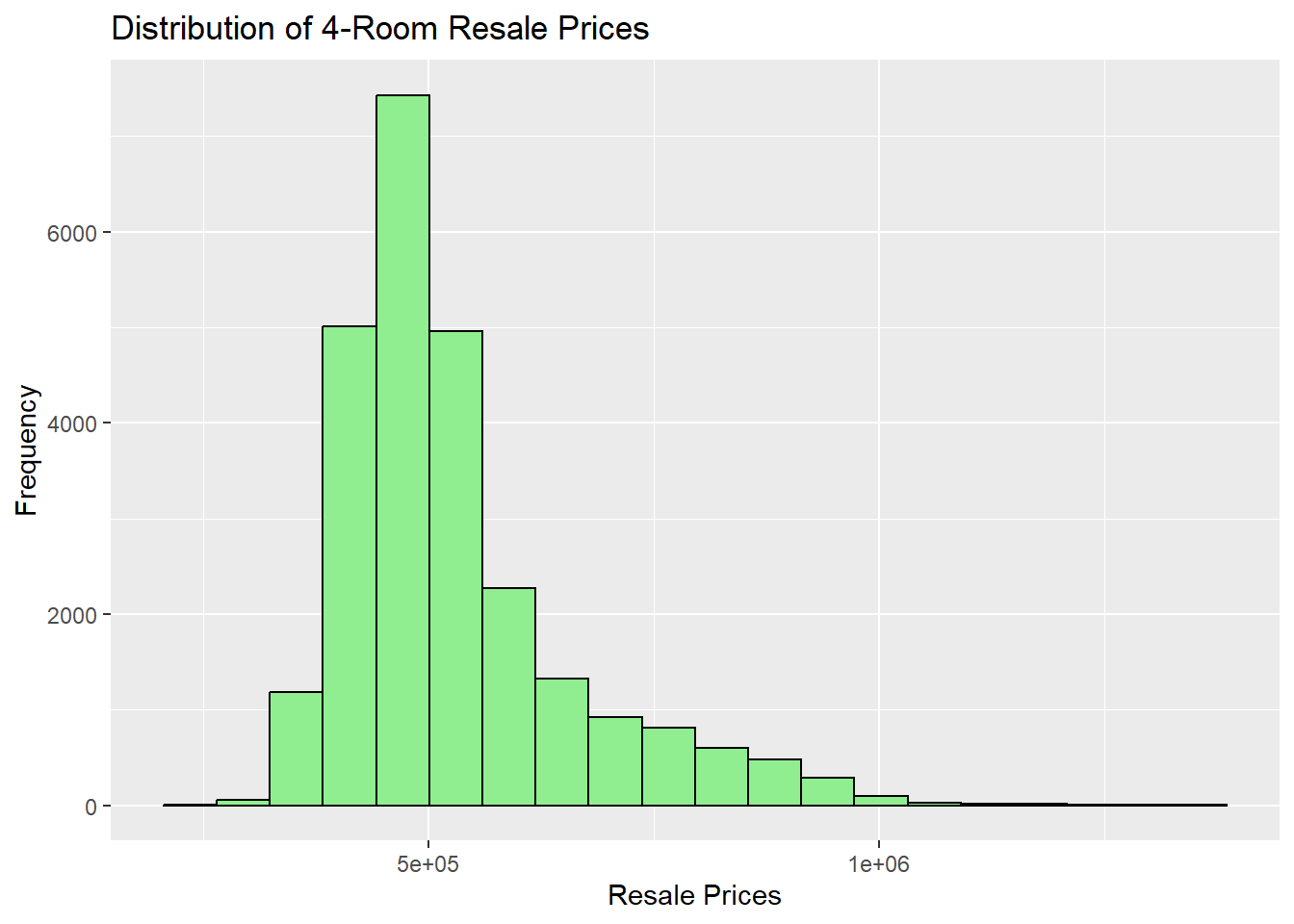

Analysis:

Based on the above graph, the histogram is skewed towards the right, meaning that 4-room HDB flats were sold at relatively lower prices.

4.2.2 Boxplots - Distribution of 4-Room Resale Prices

ggplot(data = resale_main_sf, aes(x = '', y = PRICE)) +
  geom_boxplot() +
  labs(x = '', y = 'Resale Prices')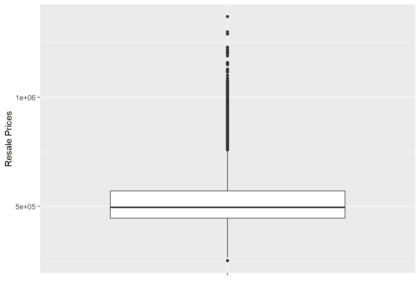

summary(resale_main_sf$PRICE)

   Min. 1st Qu.  Median    Mean 3rd Qu.    Max. 
 250000  445000  495000  529142  570000 1370000 

Analysis:

   Min. 1st Qu.  Median    Mean 3rd Qu.    Max. 
 250000  445000  495000  529142  570000 1370000 

From the graph above, it is clear that there’s a number of outliers at the higher end, and there’s one at the lower end. Most 4-rooms are sold between $445,000 to $570,000, with the lowest sold at $250,000 and the highest at $1,370,000.

4.2.3 Multiple Histogram Plots Distribution of Locational Factors

AREA_SQM <- ggplot(data = resale_main_sf, aes(x = `AREA_SQM`)) +
  geom_histogram(bins = 20, color = "black", fill = "light green")

LEASE_MTHS <- ggplot(data = resale_main_sf, aes(x = `LEASE_MTHS`)) +
  geom_histogram(bins = 20, color = "black", fill = "light green")

PROX_CBD <- ggplot(data = resale_main_sf, aes(x = `PROX_CBD`)) +
  geom_histogram(bins = 20, color = "black", fill = "light green")

PROX_BUS <- ggplot(data = resale_main_sf, aes(x = `PROX_BUS`)) +
  geom_histogram(bins = 20, color = "black", fill = "light green")

PROX_CHILDCARE <- ggplot(data = resale_main_sf, aes(x = `PROX_CHILDCARE`)) +
  geom_histogram(bins = 20, color = "black", fill = "light green")

PROX_ELDERCARE <- ggplot(data = resale_main_sf, aes(x = `PROX_ELDERCARE`)) +
  geom_histogram(bins = 20, color = "black", fill = "light green")

PROX_HAWKER <- ggplot(data = resale_main_sf, aes(x = `PROX_HAWKER`)) +
  geom_histogram(bins = 20, color = "black", fill = "light green")

PROX_GOODPRIMARY <- ggplot(data = resale_main_sf, aes(x = `PROX_GOODPRIMARY`)) +
  geom_histogram(bins = 20, color = "black", fill = "light green")

PROX_PARK <- ggplot(data = resale_main_sf, aes(x = `PROX_PARK`)) +
  geom_histogram(bins = 20, color = "black", fill = "light green")

PROX_SUPERMARKET <- ggplot(data = resale_main_sf, aes(x = `PROX_SUPERMARKET`)) +
  geom_histogram(bins = 20, color = "black", fill = "light green")

PROX_SHOPPING <- ggplot(data = resale_main_sf, aes(x = `PROX_SHOPPING`)) +
  geom_histogram(bins = 20, color = "black", fill = "light green")

PROX_MRT <- ggplot(data = resale_main_sf, aes(x = `PROX_MRT`)) +
  geom_histogram(bins = 20, color = "black", fill = "light green")

ggarrange(AREA_SQM, LEASE_MTHS, PROX_CBD, PROX_BUS, PROX_CHILDCARE, PROX_ELDERCARE, PROX_HAWKER, PROX_GOODPRIMARY, PROX_PARK, PROX_SUPERMARKET, PROX_SHOPPING, PROX_MRT, ncol = 3, nrow = 4)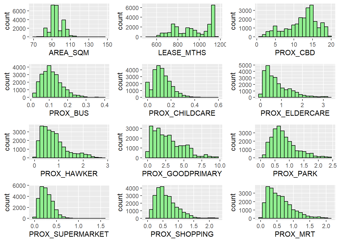

4.2.3 Multiple Histogram Plots Distribution of Locational Factors With Radius

WITHIN_350M_KINDERGARTEN <- ggplot(data = resale_main_sf, aes(x = `WITHIN_350M_KINDERGARTEN`)) +
  geom_histogram(bins = 20, color = "black", fill = "light green")

WITHIN_350M_CHILDCARE <- ggplot(data = resale_main_sf, aes(x = `WITHIN_350M_CHILDCARE`)) +
  geom_histogram(bins = 20, color = "black", fill = "light green")

WITHIN_350M_BUS <- ggplot(data = resale_main_sf, aes(x = `WITHIN_350M_BUS`)) +
  geom_histogram(bins = 20, color = "black", fill = "light green")

WITHIN_1KM_PRIMARY <- ggplot(data = resale_main_sf, aes(x = `WITHIN_1KM_PRIMARY`)) +
  geom_histogram(bins = 20, color = "black", fill = "light green")

ggarrange(WITHIN_350M_KINDERGARTEN, WITHIN_350M_CHILDCARE, WITHIN_350M_BUS, WITHIN_1KM_PRIMARY, ncol = 2, nrow = 2)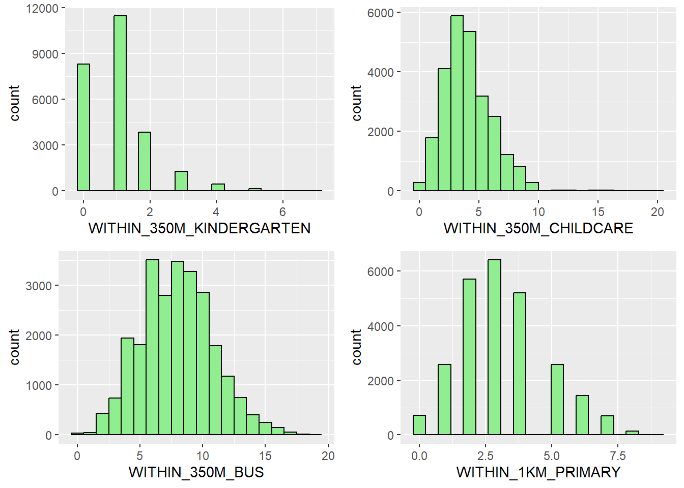

4.2.4 Point Map

tmap_mode("view")
tmap_options(check.and.fix = TRUE)
tm_shape(resale_main_sf)+
  tm_dots(col = "PRICE",
          alpha = 0.6,
          style = "quantile",
             popup.vars=c("block"="block", "street_name"="street_name", "flat_model" = "flat_model", "town" = "town", "PRICE" = "PRICE", "LEASE_MTHS", "LEASE_MTHS")) +
  tm_view(set.zoom.limits = c(11, 16))

From the above, it seems that the concentration of higher resale price for 4-room is located either the Central Area or Southern Area of Singapore

town_mean <- aggregate(resale_main_sf[, "PRICE"], list(resale_main_sf$town), mean)
town_top10 = top_n(town_mean, 10, `PRICE`) %>%
  arrange(desc(`PRICE`))
town_top10

Simple feature collection with 10 features and 2 fields
Geometry type: MULTIPOINT
Dimension:     XY
Bounding box:  xmin: 19536.43 ymin: 28217.39 xmax: 35958.92 ymax: 41493.47
Projected CRS: SVY21 / Singapore TM
           Group.1    PRICE                       geometry
1     CENTRAL AREA 857591.2 MULTIPOINT ((28640.73 29932...
2       QUEENSTOWN 783287.3 MULTIPOINT ((22133.07 32910...
3      BUKIT MERAH 717229.0 MULTIPOINT ((25024.14 28462...
4  KALLANG/WHAMPOA 703112.0 MULTIPOINT ((19536.43 41493...
5        TOA PAYOH 655306.9 MULTIPOINT ((29021.66 34720...
6         CLEMENTI 646121.4 MULTIPOINT ((19863.73 32474...
7      BUKIT TIMAH 638823.0 MULTIPOINT ((21224.71 35657...
8           BISHAN 609267.0 MULTIPOINT ((27638.13 37842...
9          GEYLANG 590617.2 MULTIPOINT ((32749.43 33252...
10      ANG MO KIO 558339.2 MULTIPOINT ((28070.74 38987...

Analysis:

From the above, it is clear that my analysis initially was correct, with Central Area being the most concentrated of higher resale price for 4-room at $857,591and Queenstown right behind at $783,287.

5 Multiple Linear Regression Method

5.1 Visualising The Relationships of The Independent Variables

Using the correlation matrix to examine if there is sign of multicolinearity.

resale_main_nogeo <- resale_main_sf %>%
  st_drop_geometry() %>%
  dplyr::select(c(7, 8, 11, 12, 14:27)) %>%
  mutate(STOREY = as.character(STOREY))

glimpse(resale_main_nogeo)

Rows: 25,502
Columns: 18
$ STOREY                   <chr> "04 TO 06", "01 TO 03", "01 TO 03", "07 TO 09…
$ AREA_SQM                 <dbl> 92, 92, 91, 92, 92, 98, 92, 92, 92, 92, 92, 1…
$ LEASE_MTHS               <dbl> 708, 693, 702, 695, 689, 681, 661, 682, 692, …
$ PRICE                    <dbl> 370000, 375000, 380000, 385000, 410000, 41000…
$ PROX_CBD                 <dbl> 9.564575, 8.401690, 9.516492, 8.580908, 9.084…
$ PROX_BUS                 <dbl> 0.16157609, 0.16740841, 0.07424143, 0.0887911…
$ PROX_CHILDCARE           <dbl> 2.493662e-01, 6.715056e-02, 1.385583e-01, 1.4…
$ PROX_ELDERCARE           <dbl> 1.08567795, 0.15039052, 0.72242472, 0.0981628…
$ PROX_HAWKER              <dbl> 0.4442515, 0.2050009, 0.4495734, 0.3190679, 0…
$ PROX_GOODPRIMARY         <dbl> 3.182527, 2.354024, 2.414729, 2.699653, 2.648…
$ PROX_PARK                <dbl> 0.8291527, 0.7847864, 0.3796058, 0.9242129, 0…
$ PROX_SUPERMARKET         <dbl> 0.4184204, 0.1946009, 0.4435109, 0.4269715, 0…
$ PROX_SHOPPING            <dbl> 1.1817959, 0.8444986, 0.2966736, 0.9304149, 0…
$ PROX_MRT                 <dbl> 1.0731215, 0.8245176, 0.4544926, 0.9503956, 0…
$ WITHIN_350M_KINDERGARTEN <dbl> 1, 0, 1, 1, 1, 0, 1, 1, 0, 0, 1, 1, 1, 1, 1, …
$ WITHIN_350M_CHILDCARE    <dbl> 2, 3, 3, 3, 3, 2, 6, 3, 3, 3, 3, 3, 5, 2, 3, …
$ WITHIN_350M_BUS          <dbl> 4, 7, 10, 4, 8, 2, 8, 7, 6, 7, 7, 7, 8, 8, 11…
$ WITHIN_1KM_PRIMARY       <dbl> 1, 3, 2, 3, 2, 2, 3, 2, 3, 3, 1, 2, 3, 2, 2, …

corrplot(cor(resale_main_nogeo[, 2:18]), diag = FALSE, order = "AOE",
         t1.pos = "td",
         t1.cex = 0.5,
         method = "number",
         type = "upper")

Analysis:

From above, there a few correlated variables and it’s within the acceptable range. All variables can be included in the regression.

5.2 Preparing Publication Quality Table: olsrr method

The code chunk below using lm() to calibrate the multiple linear regression model

resale.mlr <- lm(formula = PRICE ~ STOREY + AREA_SQM + PROX_BUS + PROX_CBD +
                   PROX_CHILDCARE + PROX_ELDERCARE + PROX_GOODPRIMARY +
                   PROX_HAWKER + PROX_MRT + PROX_PARK + PROX_SHOPPING +
                   PROX_SUPERMARKET + WITHIN_1KM_PRIMARY + WITHIN_350M_BUS +
                   WITHIN_350M_CHILDCARE + WITHIN_350M_KINDERGARTEN + LEASE_MTHS,
                 data = resale_main_nogeo)
summary(resale.mlr)

Call:
lm(formula = PRICE ~ STOREY + AREA_SQM + PROX_BUS + PROX_CBD + 
    PROX_CHILDCARE + PROX_ELDERCARE + PROX_GOODPRIMARY + PROX_HAWKER + 
    PROX_MRT + PROX_PARK + PROX_SHOPPING + PROX_SUPERMARKET + 
    WITHIN_1KM_PRIMARY + WITHIN_350M_BUS + WITHIN_350M_CHILDCARE + 
    WITHIN_350M_KINDERGARTEN + LEASE_MTHS, data = resale_main_nogeo)

Residuals:
    Min      1Q  Median      3Q     Max 
-366081  -45763   -1688   44765  366746 

Coefficients:
                           Estimate Std. Error  t value Pr(>|t|)    
(Intercept)              120014.669   8258.128   14.533  < 2e-16 ***
STOREY04 TO 06            18174.045   1415.338   12.841  < 2e-16 ***
STOREY07 TO 09            33293.452   1433.951   23.218  < 2e-16 ***
STOREY10 TO 12            42205.423   1465.693   28.796  < 2e-16 ***
STOREY13 TO 15            46506.923   1732.282   26.847  < 2e-16 ***
STOREY16 TO 18            57642.699   2237.856   25.758  < 2e-16 ***
STOREY19 TO 21            81000.888   3229.399   25.082  < 2e-16 ***
STOREY22 TO 24            93152.163   3729.839   24.975  < 2e-16 ***
STOREY25 TO 27           129017.648   4162.388   30.996  < 2e-16 ***
STOREY28 TO 30           191972.634   5073.291   37.840  < 2e-16 ***
STOREY31 TO 33           200784.072   6147.604   32.661  < 2e-16 ***
STOREY34 TO 36           229694.831   6128.617   37.479  < 2e-16 ***
STOREY37 TO 39           237916.273   7247.254   32.828  < 2e-16 ***
STOREY40 TO 42           254342.952  10061.970   25.278  < 2e-16 ***
STOREY43 TO 45           306318.117  13356.989   22.933  < 2e-16 ***
STOREY46 TO 48           363573.767  22972.861   15.826  < 2e-16 ***
STOREY49 TO 51           486732.032  39689.742   12.263  < 2e-16 ***
AREA_SQM                   3337.357     66.666   50.061  < 2e-16 ***
PROX_BUS                    560.743   8367.314    0.067   0.9466    
PROX_CBD                 -16334.883    157.010 -104.037  < 2e-16 ***
PROX_CHILDCARE           -28447.588   5842.370   -4.869 1.13e-06 ***
PROX_ELDERCARE            -7618.521    766.757   -9.936  < 2e-16 ***
PROX_GOODPRIMARY          -1106.698    276.047   -4.009 6.11e-05 ***
PROX_HAWKER              -22254.694    912.079  -24.400  < 2e-16 ***
PROX_MRT                 -23445.396   1273.357  -18.412  < 2e-16 ***
PROX_PARK                  2133.165   1051.654    2.028   0.0425 *  
PROX_SHOPPING            -24191.278   1462.249  -16.544  < 2e-16 ***
PROX_SUPERMARKET           8280.425   2994.998    2.765   0.0057 ** 
WITHIN_1KM_PRIMARY        -9076.876    341.628  -26.569  < 2e-16 ***
WITHIN_350M_BUS            1086.401    169.483    6.410 1.48e-10 ***
WITHIN_350M_CHILDCARE     -3914.981    256.907  -15.239  < 2e-16 ***
WITHIN_350M_KINDERGARTEN   6513.794    468.411   13.906  < 2e-16 ***
LEASE_MTHS                  359.103      3.123  114.989  < 2e-16 ***
---
Signif. codes:  0 '***' 0.001 '**' 0.01 '*' 0.05 '.' 0.1 ' ' 1

Residual standard error: 68620 on 25469 degrees of freedom
Multiple R-squared:  0.722, Adjusted R-squared:  0.7216 
F-statistic:  2067 on 32 and 25469 DF,  p-value: < 2.2e-16

resale.mlr <- lm(formula = PRICE ~ STOREY + AREA_SQM + PROX_BUS + PROX_CBD +
                   PROX_CHILDCARE + PROX_ELDERCARE + PROX_GOODPRIMARY +
                   PROX_HAWKER + PROX_MRT + PROX_PARK + PROX_SHOPPING +
                   PROX_SUPERMARKET + WITHIN_1KM_PRIMARY + WITHIN_350M_BUS +
                   WITHIN_350M_CHILDCARE + WITHIN_350M_KINDERGARTEN + LEASE_MTHS,
                 data = resale_main_nogeo)
ols_regress(resale.mlr)

                            Model Summary                              
----------------------------------------------------------------------
R                       0.850       RMSE                    68623.970 
R-Squared               0.722       Coef. Var                  12.969 
Adj. R-Squared          0.722       MSE                4709249303.857 
Pred R-Squared          0.721       MAE                     53943.596 
----------------------------------------------------------------------
 RMSE: Root Mean Square Error 
 MSE: Mean Square Error 
 MAE: Mean Absolute Error 

                                     ANOVA                                       
--------------------------------------------------------------------------------
                    Sum of                                                      
                   Squares           DF       Mean Square       F          Sig. 
--------------------------------------------------------------------------------
Regression    3.114971e+14           32      9.734283e+12    2067.056    0.0000 
Residual      1.199399e+14        25469    4709249303.857                       
Total         4.314369e+14        25501                                         
--------------------------------------------------------------------------------

                                                Parameter Estimates                                                 
-------------------------------------------------------------------------------------------------------------------
                   model          Beta    Std. Error    Std. Beta       t         Sig          lower         upper 
-------------------------------------------------------------------------------------------------------------------
             (Intercept)    120014.669      8258.128                   14.533    0.000    103828.267    136201.072 
          STOREY04 TO 06     18174.045      1415.338        0.057      12.841    0.000     15399.902     20948.188 
          STOREY07 TO 09     33293.452      1433.951        0.103      23.218    0.000     30482.826     36104.078 
          STOREY10 TO 12     42205.423      1465.693        0.126      28.796    0.000     39332.581     45078.266 
          STOREY13 TO 15     46506.923      1732.282        0.111      26.847    0.000     43111.552     49902.294 
          STOREY16 TO 18     57642.699      2237.856        0.098      25.758    0.000     53256.374     62029.024 
          STOREY19 TO 21     81000.888      3229.399        0.089      25.082    0.000     74671.081     87330.694 
          STOREY22 TO 24     93152.163      3729.839        0.088      24.975    0.000     85841.465    100462.861 
          STOREY25 TO 27    129017.648      4162.388        0.108      30.996    0.000    120859.129    137176.166 
          STOREY28 TO 30    191972.634      5073.291        0.130      37.840    0.000    182028.693    201916.575 
          STOREY31 TO 33    200784.072      6147.604        0.111      32.661    0.000    188734.416    212833.727 
          STOREY34 TO 36    229694.831      6128.617        0.128      37.479    0.000    217682.391    241707.271 
          STOREY37 TO 39    237916.273      7247.254        0.111      32.828    0.000    223711.240    252121.305 
          STOREY40 TO 42    254342.952     10061.970        0.085      25.278    0.000    234620.916    274064.988 
          STOREY43 TO 45    306318.117     13356.989        0.077      22.933    0.000    280137.656    332498.579 
          STOREY46 TO 48    363573.767     22972.861        0.053      15.826    0.000    318545.648    408601.887 
          STOREY49 TO 51    486732.032     39689.742        0.041      12.263    0.000    408937.869    564526.194 
                AREA_SQM      3337.357        66.666        0.176      50.061    0.000      3206.688      3468.027 
                PROX_BUS       560.743      8367.314        0.000       0.067    0.947    -15839.670     16961.157 
                PROX_CBD    -16334.883       157.010       -0.528    -104.037    0.000    -16642.633    -16027.134 
          PROX_CHILDCARE    -28447.588      5842.370       -0.017      -4.869    0.000    -39898.967    -16996.208 
          PROX_ELDERCARE     -7618.521       766.757       -0.036      -9.936    0.000     -9121.409     -6115.634 
        PROX_GOODPRIMARY     -1106.698       276.047       -0.017      -4.009    0.000     -1647.766      -565.631 
             PROX_HAWKER    -22254.694       912.079       -0.090     -24.400    0.000    -24042.421    -20466.967 
                PROX_MRT    -23445.396      1273.357       -0.068     -18.412    0.000    -25941.248    -20949.544 
               PROX_PARK      2133.165      1051.654        0.007       2.028    0.043        71.864      4194.466 
           PROX_SHOPPING    -24191.278      1462.249       -0.066     -16.544    0.000    -27057.370    -21325.187 
        PROX_SUPERMARKET      8280.425      2994.998        0.010       2.765    0.006      2410.059     14150.791 
      WITHIN_1KM_PRIMARY     -9076.876       341.628       -0.111     -26.569    0.000     -9746.487     -8407.265 
         WITHIN_350M_BUS      1086.401       169.483        0.024       6.410    0.000       754.205      1418.598 
   WITHIN_350M_CHILDCARE     -3914.981       256.907       -0.060     -15.239    0.000     -4418.533     -3411.428 
WITHIN_350M_KINDERGARTEN      6513.794       468.411        0.049      13.906    0.000      5595.682      7431.906 
              LEASE_MTHS       359.103         3.123        0.455     114.989    0.000       352.982       365.224 
-------------------------------------------------------------------------------------------------------------------

5.3 Preparing Publication Quality Table: gtsummary method

tbl_regression(resale.mlr, intercept = TRUE)

Characteristic	Beta	95% CI1	p-value
(Intercept)	120,015	103,828, 136,201	<0.001
STOREY
01 TO 03	—	—
04 TO 06	18,174	15,400, 20,948	<0.001
07 TO 09	33,293	30,483, 36,104	<0.001
10 TO 12	42,205	39,333, 45,078	<0.001
13 TO 15	46,507	43,112, 49,902	<0.001
16 TO 18	57,643	53,256, 62,029	<0.001
19 TO 21	81,001	74,671, 87,331	<0.001
22 TO 24	93,152	85,841, 100,463	<0.001
25 TO 27	129,018	120,859, 137,176	<0.001
28 TO 30	191,973	182,029, 201,917	<0.001
31 TO 33	200,784	188,734, 212,834	<0.001
34 TO 36	229,695	217,682, 241,707	<0.001
37 TO 39	237,916	223,711, 252,121	<0.001
40 TO 42	254,343	234,621, 274,065	<0.001
43 TO 45	306,318	280,138, 332,499	<0.001
46 TO 48	363,574	318,546, 408,602	<0.001
49 TO 51	486,732	408,938, 564,526	<0.001
AREA_SQM	3,337	3,207, 3,468	<0.001
PROX_BUS	561	-15,840, 16,961	>0.9
PROX_CBD	-16,335	-16,643, -16,027	<0.001
PROX_CHILDCARE	-28,448	-39,899, -16,996	<0.001
PROX_ELDERCARE	-7,619	-9,121, -6,116	<0.001
PROX_GOODPRIMARY	-1,107	-1,648, -566	<0.001
PROX_HAWKER	-22,255	-24,042, -20,467	<0.001
PROX_MRT	-23,445	-25,941, -20,950	<0.001
PROX_PARK	2,133	72, 4,194	0.043
PROX_SHOPPING	-24,191	-27,057, -21,325	<0.001
PROX_SUPERMARKET	8,280	2,410, 14,151	0.006
WITHIN_1KM_PRIMARY	-9,077	-9,746, -8,407	<0.001
WITHIN_350M_BUS	1,086	754, 1,419	<0.001
WITHIN_350M_CHILDCARE	-3,915	-4,419, -3,411	<0.001
WITHIN_350M_KINDERGARTEN	6,514	5,596, 7,432	<0.001
LEASE_MTHS	359	353, 365	<0.001
1 CI = Confidence Interval

5.4 Checking for Multicolinearity

ols_vif_tol(resale.mlr)

                  Variables Tolerance      VIF
1            STOREY04 TO 06 0.5453259 1.833766
2            STOREY07 TO 09 0.5526886 1.809337
3            STOREY10 TO 12 0.5661245 1.766396
4            STOREY13 TO 15 0.6433468 1.554372
5            STOREY16 TO 18 0.7594335 1.316771
6            STOREY19 TO 21 0.8589673 1.164189
7            STOREY22 TO 24 0.8859272 1.128761
8            STOREY25 TO 27 0.9019700 1.108684
9            STOREY28 TO 30 0.9220648 1.084522
10           STOREY31 TO 33 0.9418010 1.061795
11           STOREY34 TO 36 0.9406107 1.063139
12           STOREY37 TO 39 0.9573717 1.044526
13           STOREY40 TO 42 0.9708734 1.030000
14           STOREY43 TO 45 0.9786577 1.021808
15           STOREY46 TO 48 0.9918187 1.008249
16           STOREY49 TO 51 0.9966094 1.003402
17                 AREA_SQM 0.8811246 1.134913
18                 PROX_BUS 0.8620575 1.160015
19                 PROX_CBD 0.4244658 2.355902
20           PROX_CHILDCARE 0.8721396 1.146605
21           PROX_ELDERCARE 0.8365748 1.195350
22         PROX_GOODPRIMARY 0.5928120 1.686875
23              PROX_HAWKER 0.8029681 1.245380
24                 PROX_MRT 0.8000420 1.249934
25                PROX_PARK 0.8580656 1.165412
26            PROX_SHOPPING 0.6879710 1.453550
27         PROX_SUPERMARKET 0.8865753 1.127936
28       WITHIN_1KM_PRIMARY 0.6199215 1.613107
29          WITHIN_350M_BUS 0.7671970 1.303446
30    WITHIN_350M_CHILDCARE 0.7114620 1.405556
31 WITHIN_350M_KINDERGARTEN 0.8882120 1.125857
32               LEASE_MTHS 0.6974027 1.433892

Analysis:

Since the VIF of the independent variables are less than 10, it is safe to say that there are no sign of multicollinearity among the independent variables.

5.5 Test for Non-Linearity

ols_plot_resid_fit(resale.mlr)

Analysis:

From the figure above, most of the data points are scattered around the 0 line. This shows that the relationship between the dependent variable and the independent variables are linear.

5.6 Test for Normality Assumption

ols_plot_resid_hist(resale.mlr)

Analysis:

From the figure above, it shows that the residual of the multiple linear regression model is normally distributed.

5.7 Testing for Spatial Autocorrelation

5.7.1 Export the Residual and Save as a Data Frame

mlr.output <- as.data.frame(resale.mlr$residuals)

5.7.2 Join Data Frame with resale_main_sf Object

resale.res.sf <- cbind(resale_main_sf,
                       resale.mlr$residuals) %>%
  rename(`MLR_RES` = resale.mlr.residuals)

5.7.3 Convert from sf to sp

resale.sp <- as_Spatial(resale.res.sf)
resale.sp

class       : SpatialPointsDataFrame 
features    : 25502 
extent      : 11519.79, 42645.18, 28217.39, 48741.06  (xmin, xmax, ymin, ymax)
crs         : +proj=tmerc +lat_0=1.36666666666667 +lon_0=103.833333333333 +k=1 +x_0=28001.642 +y_0=38744.572 +ellps=WGS84 +towgs84=0,0,0,0,0,0,0 +units=m +no_defs 
variables   : 28
names       :   month,       town,          address, block,   street_name, flat_type,   STOREY, AREA_SQM,    flat_model, lease_commence_date, LEASE_MTHS,   PRICE, postal,          PROX_CBD,           PROX_BUS, ... 
min values  : 2021-01, ANG MO KIO,   1 CHAI CHEE RD,     1,  ADMIRALTY DR,    4 ROOM, 01 TO 03,       70, Adjoined flat,                1967,        517,  250000, 052335, 0.999393538715878, 0.0158480216214286, ... 
max values  : 2023-02,     YISHUN, 9B BOON TIONG RD,    9B, YUNG SHENG RD,    4 ROOM, 49 TO 51,      145,       Type S1,                2019,       1168, 1370000,    NIL,  19.6500691667807,  0.391470769487539, ... 

5.7.4 Visualise the Distribution of Residuals

tm_shape(mpsz)+
  tmap_options(check.and.fix = TRUE) +
  tm_polygons(alpha = 0.4) +
tm_shape(resale.res.sf) +  
  tm_dots(col = "MLR_RES",
          alpha = 0.6,
          style="quantile") +
  tm_view(set.zoom.limits = c(11,14))

5.8 Moran’s I Test

5.8.1 Computing Distance-Based Weight Matrix

nb <- dnearneigh(coordinates(resale.sp), 0, 1500, longlat = FALSE)
summary(nb)

Neighbour list object:
Number of regions: 25502 
Number of nonzero links: 26961048 
Percentage nonzero weights: 4.145609 
Average number of links: 1057.213 
Link number distribution:

   5   28   33   40   85   88   91   93  111  112  135  150  153  155  156  162 
   6   29   25    9    3   84   11    5    1    3    3  129   19    3    1    1 
 164  167  168  172  179  181  184  185  193  195  197  198  199  200  201  203 
   1    2    5    3    5    5    1    1   10    3   10    6   20    2   48    5 
 204  205  206  208  210  211  212  214  215  217  218  219  220  221  222  223 
   5   91   15   21    1    3    1   13   13    8    5    2   29    8    3   14 
 224  226  227  228  230  232  234  235  236  238  239  240  241  242  243  244 
   6    5   41   15    2   18   19    1   17    6    6    6   17   18    8    4 
 245  246  247  248  249  250  251  252  254  256  257  258  259  260  262  263 
  39   10   26   35    7    2    9   14   26    7   25    3    2    2   28   24 
 264  265  266  267  268  269  270  271  272  273  274  275  276  277  278  279 
  36   13   16   10   17   22    2   12   21   17    9    5   22   14    9   24 
 280  281  282  283  284  285  286  287  289  290  291  292  293  294  295  296 
  17    6   36   13   50    3   31   21   16   10    9   33   11   11    8   12 
 297  298  299  300  301  302  306  307  308  310  311  312  313  314  315  316 
  40   57   29    6   26   11   14    5   18    4    9    9    8    7   32   10 
 317  318  319  320  321  322  323  324  325  326  327  328  329  330  331  332 
  46   14    6   15   13    9   15   19   13    7   12   50    5    6   32    7 
 333  334  335  336  337  338  339  340  341  342  343  344  345  346  347  348 
   8   43    7   15    7   14    6   12   11   20   15    6    5   25   13    9 
 349  350  351  352  353  354  355  356  357  358  359  360  361  362  363  364 
  13   14   16    3   19    8    6   16    6   14    7   17    7   27    9    2 
 365  366  367  368  369  370  371  372  373  374  375  376  377  378  379  380 
   2   18   31   13    9   39   23   13    8   23   26   10   16    5    6   16 
 382  383  384  385  386  387  388  389  390  391  392  393  394  395  396  397 
   8    9    2   13   14   11   18   32   32    7   18   12    8   17   33    4 
 398  399  400  401  402  403  404  405  406  407  408  409  410  411  412  413 
  16   12    4   39   19    6   25   11   19   33   19   58   16   27    4    7 
 414  415  416  417  418  419  420  421  422  423  424  425  426  427  428  429 
   4    5   30   19   34   13   10    9   29   16   14   10   13   23    6   30 
 430  431  432  433  434  435  436  437  438  439  440  441  442  443  444  445 
  18   18   20    9   13   15   18   10   31    8    9    6   16   25   17   29 
 446  447  448  449  450  451  452  453  454  455  456  457  458  459  460  461 
  20   17   28   16    7   28    9   43   20   40   27   20   22    7   45   24 
 462  463  464  465  466  467  468  469  470  471  472  473  474  475  476  477 
  27   20   51   13   19    3    8   16   10   16   11   17   52   20   65   14 
 478  479  480  481  482  483  484  485  486  487  488  489  490  491  492  493 
  14   17   20   21   70   31  107   22   24   15   30   14   11   16   30    9 
 494  495  496  497  498  499  500  501  502  503  504  505  506  507  508  509 
  27   12    4   20   24   18   18   23   19   22   10   15   16    3    9   15 
 510  511  512  513  514  515  516  517  518  519  520  521  522  523  524  525 
   3   10   15   29    8    6   26   12    6    7   54   21   15    7   16   16 
 526  527  528  529  530  531  532  533  534  535  536  537  538  539  540  541 
  10    9   23   39   15   29   47    8   14   20   16   22    9   19   35   48 
 542  543  544  545  546  547  548  549  550  551  552  553  554  555  556  557 
  45   27    6   21   14   32   24   15   15    8   80   13    8   40   13    8 
 558  559  560  561  562  563  564  565  566  567  568  569  570  571  572  573 
  32   27   24   18   16    5   25   54   11   27    8   48    6   34   18   10 
 574  575  576  577  578  579  580  581  582  583  584  585  586  587  588  589 
  36   14   31   10   16   40   22   14   48   39   67   20   24   24   25   18 
 590  591  592  593  594  595  596  597  598  599  600  601  602  603  604  605 
  29   22   22   18   23    5   32   13   18   22   27   21    7   38   12   22 
 606  607  608  609  610  611  612  613  614  615  616  617  618  619  620  621 
  22   23   49   35   27   10   13   22   41    7   20   18   12   18   31   80 
 622  623  624  625  626  627  628  629  630  631  632  633  634  635  636  637 
  53   27   67    7   47   18   22    1   22   27   15    8   25   47   47   13 
 638  639  640  641  642  643  644  645  646  647  648  649  650  651  652  653 
  36   18   25   11   14   22   40   25   35   35   66   88    2   73   19   14 
 654  655  656  657  658  659  660  661  662  663  664  665  666  667  668  669 
   6   16   30   22   20   22    5   17   13   43   16   10   17   25   20   33 
 670  671  672  673  674  675  676  677  678  679  680  681  682  683  684  685 
  62   19    9   30   31   13   17    8   19   28   17   10   43   17   13   15 
 686  687  688  689  690  691  692  693  694  695  696  697  698  699  700  701 
   7    8   24   18   19   25   40   59   42   30   13   31   25    7   18   20 
 702  703  704  705  706  707  708  709  710  711  712  713  714  715  716  717 
  56   34   39   32   64   31   19   23   33   19   35   42   12   15   21    7 
 718  719  720  721  722  723  724  725  726  727  728  729  730  731  732  733 
  11   11    5   16   11    9    7   29   32   35    8   30    4   10   18    1 
 734  735  736  737  738  739  740  741  742  743  744  745  746  747  748  749 
   5   17   17    8   22   39   15    5   12   28   44    8   21   43    7   17 
 750  751  752  753  754  755  756  757  758  759  760  761  762  763  764  765 
   5   24   46   42   10   47    6   19   41   10    8    7   14   21   27    7 
 766  767  768  769  770  771  772  773  774  775  776  777  779  780  781  782 
  14    4    6   33    6    4   27   15   23   26   23   22   34    6   10    5 
 783  784  785  786  787  788  789  790  791  792  793  794  795  796  797  798 
   6    7   22   41   15   27   34   15    2    2    9   20   41   20    7   20 
 799  800  801  802  803  804  805  806  807  808  809  810  812  813  814  815 
  10   12    6   43    7   17   12   11    9   13   22    4    8   14   11   16 
 816  817  818  820  821  822  823  824  825  826  827  829  830  831  832  833 
   8   24    5    2    3    8    4    2    3   35   18   14   12    8    5    1 
 834  835  836  837  839  840  841  842  843  844  845  846  847  848  849  850 
  24    8   49    6   20    2   15    9   16   13    3   12   17    4   12    8 
 851  852  854  855  857  858  859  860  861  863  864  865  866  868  869  870 
   5   21    8    7    4    2    8   10   14   22    9    9   15   21    7   13 
 872  873  874  875  876  877  878  879  880  881  882  883  884  885  886  887 
   6   12    1   10    4   24   14   31   51   21    8   51   15    1    3   12 
 888  889  890  891  892  893  894  895  896  898  899  900  901  902  903  904 
  14    4   21   33   14    6   32    4   22    7   20   29    7    7   33   12 
 905  907  908  909  910  911  912  913  914  915  916  917  918  919  920  921 
  13   10    3    3   15   14    8   10    7   28    2    6   14    5   29   29 
 922  923  924  925  926  927  928  929  930  931  932  933  934  935  936  937 
  16   29    2    3   22   15    3    3    7   24    9   19   26   13   12   17 
 938  939  940  941  942  943  944  945  946  947  948  949  950  951  952  953 
  12    6   37   39   10   10   10   13   21   15   21   10   23   27    6   21 
 955  956  958  959  960  961  962  963  964  965  966  967  968  969  970  971 
   5   16   28   59   15    5   23   26    7   18    4    2    8    1   24   23 
 972  973  974  975  976  977  978  979  980  981  982  983  984  985  986  987 
   8   21   21    8   18   13   28   10   14    8    9    9    2   18    2    7 
 988  989  990  991  992  993  994  995  996  997  999 1000 1001 1002 1004 1005 
  10   15   11   12    2   11   79    8    6    6    9    1   36    7   15    6 
1006 1007 1008 1009 1010 1011 1012 1013 1014 1015 1016 1017 1018 1019 1020 1021 
  13    3   15    6   33   16   14   17   16    9   15   17   16    1   10    1 
1022 1023 1024 1025 1026 1027 1028 1030 1031 1032 1033 1034 1035 1036 1037 1038 
  19   54   17    7   13    4   23   16   25   18   15   26    1   18   19   19 
1039 1040 1041 1042 1043 1044 1045 1048 1051 1052 1053 1054 1055 1056 1057 1058 
  23    7    4    4   15    9   14   10   14   19   14    5   34   11    5   15 
1059 1060 1061 1062 1063 1064 1065 1066 1067 1068 1069 1070 1071 1072 1073 1074 
  18   10   12    8    9    6    7   24   10   19   16    6   10    8   11    3 
1075 1076 1077 1078 1079 1080 1081 1082 1083 1084 1085 1086 1087 1088 1089 1090 
  21    8   20    9   12   17    5   12   27   13   12   15   12   19   18    7 
1091 1092 1094 1095 1096 1097 1098 1099 1100 1101 1102 1104 1105 1106 1107 1108 
  45    6   11   18   38    2   10   10   13    7    8   12   17    6   16    9 
1110 1111 1112 1113 1114 1115 1116 1117 1118 1119 1120 1121 1123 1124 1125 1126 
   2    8   26   21   19   14   12   33    2   32    9   26    1   15    8   13 
1127 1128 1129 1130 1131 1132 1133 1134 1135 1136 1137 1138 1139 1140 1141 1143 
  27   33   19   10   16   29   16   19   26   19   35   22    2    1   12    9 
1144 1145 1146 1147 1148 1149 1150 1151 1152 1153 1154 1155 1156 1157 1158 1159 
   5    2   11   28   15   12    9   18    6   34    6   13   21   13    7    5 
1160 1161 1162 1163 1164 1165 1166 1167 1168 1169 1170 1171 1172 1173 1174 1175 
   7   14    9   23   17   21    9   19   11   19   24    1   25   37    7   14 
1176 1177 1178 1179 1180 1181 1182 1183 1184 1185 1186 1187 1188 1189 1190 1191 
   7   10   11    8    8   11    1   24    9    7   30   20   11    1    3   15 
1192 1193 1194 1195 1196 1197 1198 1199 1200 1201 1202 1203 1204 1205 1206 1207 
  29   28    2   23   10    7   15   11    8    4   14    5    3   21    3    7 
1208 1209 1210 1211 1212 1213 1214 1215 1216 1217 1218 1219 1221 1222 1223 1224 
  14    5    3    7   10    2   13    7    6   30   18   14   28   24   10    7 
1225 1226 1227 1228 1229 1230 1231 1232 1233 1234 1235 1236 1238 1239 1240 1241 
  19    2   34    3   14    9   12   11   10   24    2   24    3   15   20    6 
1242 1243 1244 1245 1246 1247 1248 1249 1251 1252 1253 1254 1255 1256 1257 1258 
  15   14    7    9    2    8   10    9   16    5   16   22   15   30   25   19 
1259 1260 1261 1262 1263 1264 1265 1266 1267 1269 1270 1271 1273 1274 1275 1276 
   3   17   16   29    6   12   17    1   25   35   12    1    8   19    2   10 
1277 1279 1280 1281 1282 1283 1284 1285 1286 1287 1288 1289 1290 1291 1292 1293 
  38    5    4   37    3   16    2   15   16   10   25    4   20   11   11    1 
1295 1296 1297 1298 1299 1300 1302 1303 1304 1306 1307 1308 1309 1310 1311 1313 
  17   56    5   16    5    9    4   14   22    3   29   22    7   11   12    8 
1314 1315 1316 1317 1318 1319 1320 1321 1323 1324 1325 1326 1327 1328 1329 1330 
  77   24    3   31   10   12   27    8   29   16    2   12    8   16   22    8 
1332 1333 1334 1336 1337 1338 1339 1340 1342 1343 1344 1345 1346 1347 1348 1349 
   9    1    6   28    7   40    1    6   14    7   31    9    2   56   30   24 
1350 1351 1352 1353 1354 1355 1356 1358 1359 1360 1361 1362 1363 1364 1365 1368 
   7    5   15   10    1    5   18    7   19   26   12   48   38   26   13   10 
1369 1370 1371 1372 1373 1374 1375 1376 1377 1378 1379 1381 1382 1383 1385 1386 
  13    9   35    4    4    9   15    9   13   14   11   13    1   16   20   13 
1387 1388 1389 1391 1392 1395 1396 1397 1398 1400 1401 1402 1403 1404 1405 1406 
   9    5    4   17    9   19   20    1    4   16    4    1    1   21   22   15 
1407 1408 1409 1410 1411 1412 1413 1416 1417 1418 1421 1424 1425 1426 1427 1428 
  17   14    3   14    1    3   10    7    9    3    5    3    2   13    8   21 
1429 1430 1431 1433 1434 1435 1436 1437 1438 1439 1441 1443 1444 1445 1446 1447 
  13   23    4    6    4    2   11    2    3    1    5    1    2    2   12    4 
1448 1450 1451 1452 1453 1454 1455 1456 1458 1459 1460 1462 1463 1465 1466 1467 
   8    4    2    4   11   13    3    2    6    5    2    1   10   17   15   24 
1468 1469 1470 1471 1473 1474 1475 1477 1478 1479 1480 1481 1482 1483 1484 1485 
   3    5    2    7    1   10   14    3    6    2    6    8    1    2    2    2 
1487 1489 1490 1492 1493 1494 1495 1496 1497 1499 1501 1502 1504 1505 1507 1510 
   4   18    1    2    7    1    4    1    9   14   12    1    7    7   23    4 
1513 1514 1515 1516 1517 1518 1523 1524 1525 1526 1528 1531 1532 1535 1536 1538 
  11   13    8    5   14    2    1    3    1   13    4    9   18    1    3    1 
1539 1540 1543 1544 1545 1548 1549 1551 1552 1554 1555 1556 1558 1559 1560 1565 
   3   19    2    3    9    7    6   16    7   15   24   28    3    1   14    3 
1566 1567 1568 1571 1576 1580 1582 1583 1585 1586 1587 1589 1590 1591 1593 1595 
  10    6    3    7    5    5   13    4    9    1    5    3    5   12    9    2 
1597 1599 1600 1602 1603 1604 1605 1606 1607 1608 1609 1610 1612 1615 1617 1618 
   6    3    3    6    3   13    4   11    3    3   11   14   21   13   15    2 
1619 1620 1624 1626 1630 1632 1634 1636 1637 1643 1647 1648 1649 1650 1652 1656 
   2   20    8   11   16    3   18   20   20    1   13    4   10    8    5    8 
1658 1659 1660 1662 1663 1667 1673 1674 1675 1677 1681 1684 1686 1687 1690 1697 
   1   12    1    2    8   18    4    1    1    5    4   10    1    2    8    4 
1702 1703 1705 1706 1707 1710 1715 1717 1718 1720 1721 1722 1723 1725 1727 1728 
  13    6   27    8    1   11    4    6    9    8    1    2   10    2    2    5 
1729 1731 1732 1734 1735 1737 1743 1744 1745 1746 1747 1748 1751 1754 1757 1758 
   4    2    1    3    1    4    4    6   13    1    2    3    7    8    3   10 
1759 1761 1762 1763 1764 1765 1766 1767 1768 1769 1771 1772 1773 1778 1779 1781 
   9    5    1   11    8   21    2    3    6    3    9    2    6   24    1   11 
1786 1787 1788 1789 1790 1791 1792 1793 1794 1795 1796 1799 1800 1801 1803 1804 
   3    5    6    7    4    4    1    3   16    1   10    4    8    7    2    3 
1805 1809 1811 1812 1817 1819 1820 1824 1826 1827 1829 1830 1831 1834 1836 1838 
   5    2   16    3    1    8   11    4    1    1   10   18    1   15    9    3 
1839 1840 1841 1842 1843 1845 1846 1847 1848 1849 1850 1851 1855 1856 1857 1858 
   9    5    3    6    9    6   13    8   15    1    5   11    6    9    2   11 
1859 1860 1862 1863 1864 1865 1867 1868 1869 1870 1871 1872 1873 1874 1875 1876 
   2    8   28   17    2    5    3    6    5    5    4    3    3    3    4    5 
1878 1881 1887 1889 1890 1892 1894 1896 1897 1899 1900 1905 1907 1908 1911 1912 
  23   10    4    1   18    1    4    7   22    3    4   19    1   10    7    6 
1913 1914 1915 1916 1917 1919 1922 1923 1924 1926 1929 1930 1932 1934 1935 1936 
  12    7   14    1    2   10   13    7    7    2    2    9    2   10   66    9 
1940 1941 1945 1953 1955 1958 1959 1960 1962 1963 1965 1972 1973 1976 1979 1980 
   6   12   11    4   18    4    5    5    7   12    6   11   18    7    5    6 
1982 1984 1986 1988 1989 1994 1995 2002 2003 2006 2007 2017 2025 2026 2029 2031 
  13    7    6    6    2   11    2    3   37   11    8   17    2    6   20   10 
2032 2033 2034 2035 2037 2039 2040 2042 2044 2045 2046 2047 2048 2049 2051 2054 
   3   11    5    6    4   14   26    1    2    4    3   17   12    1    7    1 
2055 2057 2063 2065 2066 2067 2068 2070 2071 2074 2075 2076 2077 2078 2080 2083 
   2   14    5   14    4    6   38   11    9    4    4   13    1   20    4   23 
2084 2085 2088 2089 2091 2092 2093 2094 2098 2100 2102 2103 2106 2108 2109 2110 
  11   34    2   13    6   17    8   10    4    7    6   19    3    1    7   18 
2111 2112 2115 2116 2118 2120 2121 2122 2123 2125 2126 2128 2131 2132 2133 2135 
   1    9   11   44    8   14   28   27    3   17   11   21   12    3   11    5 
2137 2139 2140 2141 2145 2146 2147 2148 2149 2150 2152 2153 2155 2157 2158 2160 
  19   14    3   19   17    1    1   21    3    3    8    8    7   36    4   15 
2162 2163 2164 2165 2167 2171 2172 2175 2176 2179 2180 2181 2186 2189 2191 2193 
  17    4    8    4   14    9   12   18    6    7    2    3   14    3    6   10 
2194 2195 2197 2198 2199 2203 2205 2206 2209 2212 2213 2215 2217 2220 2222 2224 
  48   18    6    1    3    5    6    8   28   11    8    5   17    6    2    3 
2227 2228 2229 2230 2234 2238 2242 2247 2249 2251 2252 2253 2254 2256 2258 2262 
   7    4   12   11    3    6    3    2   21    3    1   13    2   28    5    2 
2264 2266 2267 2271 2272 2273 2275 2276 2277 2279 2283 2287 2292 2298 2299 2301 
   2    9    1    3    3    6    2    4   16    2    6   16    2    1   50    2 
2302 2303 2305 2306 2307 2310 2315 2317 2318 2324 2328 2330 2332 2335 2337 2338 
   8    5    6    6    4    3    3    1    2    6    1    3    3    3   11    2 
2346 2349 2350 2351 2352 2354 2355 2362 2363 2366 2369 2370 2373 2374 2379 2381 
  10    4    5    4    7   11   10    2   10   22    3    1    2    7    2    2 
2385 2389 2391 2393 2395 2396 2406 2416 2417 2421 2422 2423 2424 2426 2427 2429 
   1   20    6    8   11    7    3    1   11    2    1   11    6    5    2    1 
2430 2434 2436 2438 2440 2444 2446 2447 2455 2456 2458 2460 2462 2463 2468 2473 
   3   10    3   16    5    8    3    2    6    5   14    4   28    2    4    8 
2474 2483 2491 2495 2496 2501 2510 2515 2521 2526 2531 2534 2538 2542 2547 2548 
  13   14    8    3    4   20    7    5   15    3    1    1    9   10    2    4 
2552 2561 2562 2567 2569 2576 2585 2587 2593 2597 2598 2601 2606 2609 2611 2612 
   8    2    1   15    7    7    1    9    1    9   20    7    5   11   12    6 
2617 2632 2647 2651 2653 2654 2655 2659 2665 2672 2674 2675 2678 2682 2688 2689 
  26    5    2    3    4    1    7   11    8   18    2    7    2   15   15    3 
2694 2700 2703 2710 2717 2722 2727 2730 2733 2734 2739 2744 2750 2751 2754 2755 
  16   20    4   13    6   25    3    3    2   20    2    8   14    4    6    9 
2762 2764 2765 2774 2782 2783 2788 2789 2790 2791 2792 2793 2800 2801 2803 2804 
   4    1   14   10   15    5    8   14    9   13   13    2    4    8   10    3 
2805 2811 2822 2827 2829 2830 2833 2834 2840 2841 2842 2845 2847 2852 2856 2859 
  11    4    9   10   10    4    3    1    4   10    3    1    4   18   10    5 
2864 2866 2870 2872 2877 2881 2886 2898 2900 2914 2918 2925 2926 2927 2930 2932 
   5    2   13    2    6   19    6    7    7    1    6   12    3   13    2    5 
2936 2942 2943 2950 2953 2955 2959 2967 2968 2974 2975 2976 2982 2986 2987 2994 
   5   24    1    4    2    8    9    5    5    5    6    2    3   17    4   10 
2996 3002 3007 3008 3012 3017 3026 3031 3037 3040 3054 3058 3067 3068 3069 3071 
   2   18   15    8    2    3    7    4    2    2    4    3    4    5    5    3 
3074 3076 3086 3095 3105 3111 3115 3135 3138 3139 3142 3144 3146 3155 3156 3168 
   3    2    2    5    3    9    1    3    7    2    8    6    4    2    2    6 
3175 3176 3178 3182 3185 3187 3189 3194 3196 3203 3212 3221 3229 3241 3244 3245 
   3    2    1    8    2    3    9    4    3    3    1    4   10    4   12    3 
3252 3255 3264 3265 3267 3278 3285 3291 3307 3310 3313 3317 3322 3328 3331 3333 
   3   10   10   13    4    3    6    2    4    7    2    6    1    2    1    2 
3338 3343 3357 3405 3424 3441 3452 3473 3486 
   6    2    1    1    6    4    2    1    1 
6 least connected regions:
5233 5270 5273 14652 22145 22146 with 5 links
1 most connected region:
6060 with 3486 links

5.8.2 Convert the Output Neighbours Lists into Spatial Weights

nb_lw <- nb2listw(nb, style = 'W', zero.policy = TRUE)
summary(nb_lw)

Characteristics of weights list object:
Neighbour list object:
Number of regions: 25502 
Number of nonzero links: 26961048 
Percentage nonzero weights: 4.145609 
Average number of links: 1057.213 
Link number distribution:

   5   28   33   40   85   88   91   93  111  112  135  150  153  155  156  162 
   6   29   25    9    3   84   11    5    1    3    3  129   19    3    1    1 
 164  167  168  172  179  181  184  185  193  195  197  198  199  200  201  203 
   1    2    5    3    5    5    1    1   10    3   10    6   20    2   48    5 
 204  205  206  208  210  211  212  214  215  217  218  219  220  221  222  223 
   5   91   15   21    1    3    1   13   13    8    5    2   29    8    3   14 
 224  226  227  228  230  232  234  235  236  238  239  240  241  242  243  244 
   6    5   41   15    2   18   19    1   17    6    6    6   17   18    8    4 
 245  246  247  248  249  250  251  252  254  256  257  258  259  260  262  263 
  39   10   26   35    7    2    9   14   26    7   25    3    2    2   28   24 
 264  265  266  267  268  269  270  271  272  273  274  275  276  277  278  279 
  36   13   16   10   17   22    2   12   21   17    9    5   22   14    9   24 
 280  281  282  283  284  285  286  287  289  290  291  292  293  294  295  296 
  17    6   36   13   50    3   31   21   16   10    9   33   11   11    8   12 
 297  298  299  300  301  302  306  307  308  310  311  312  313  314  315  316 
  40   57   29    6   26   11   14    5   18    4    9    9    8    7   32   10 
 317  318  319  320  321  322  323  324  325  326  327  328  329  330  331  332 
  46   14    6   15   13    9   15   19   13    7   12   50    5    6   32    7 
 333  334  335  336  337  338  339  340  341  342  343  344  345  346  347  348 
   8   43    7   15    7   14    6   12   11   20   15    6    5   25   13    9 
 349  350  351  352  353  354  355  356  357  358  359  360  361  362  363  364 
  13   14   16    3   19    8    6   16    6   14    7   17    7   27    9    2 
 365  366  367  368  369  370  371  372  373  374  375  376  377  378  379  380 
   2   18   31   13    9   39   23   13    8   23   26   10   16    5    6   16 
 382  383  384  385  386  387  388  389  390  391  392  393  394  395  396  397 
   8    9    2   13   14   11   18   32   32    7   18   12    8   17   33    4 
 398  399  400  401  402  403  404  405  406  407  408  409  410  411  412  413 
  16   12    4   39   19    6   25   11   19   33   19   58   16   27    4    7 
 414  415  416  417  418  419  420  421  422  423  424  425  426  427  428  429 
   4    5   30   19   34   13   10    9   29   16   14   10   13   23    6   30 
 430  431  432  433  434  435  436  437  438  439  440  441  442  443  444  445 
  18   18   20    9   13   15   18   10   31    8    9    6   16   25   17   29 
 446  447  448  449  450  451  452  453  454  455  456  457  458  459  460  461 
  20   17   28   16    7   28    9   43   20   40   27   20   22    7   45   24 
 462  463  464  465  466  467  468  469  470  471  472  473  474  475  476  477 
  27   20   51   13   19    3    8   16   10   16   11   17   52   20   65   14 
 478  479  480  481  482  483  484  485  486  487  488  489  490  491  492  493 
  14   17   20   21   70   31  107   22   24   15   30   14   11   16   30    9 
 494  495  496  497  498  499  500  501  502  503  504  505  506  507  508  509 
  27   12    4   20   24   18   18   23   19   22   10   15   16    3    9   15 
 510  511  512  513  514  515  516  517  518  519  520  521  522  523  524  525 
   3   10   15   29    8    6   26   12    6    7   54   21   15    7   16   16 
 526  527  528  529  530  531  532  533  534  535  536  537  538  539  540  541 
  10    9   23   39   15   29   47    8   14   20   16   22    9   19   35   48 
 542  543  544  545  546  547  548  549  550  551  552  553  554  555  556  557 
  45   27    6   21   14   32   24   15   15    8   80   13    8   40   13    8 
 558  559  560  561  562  563  564  565  566  567  568  569  570  571  572  573 
  32   27   24   18   16    5   25   54   11   27    8   48    6   34   18   10 
 574  575  576  577  578  579  580  581  582  583  584  585  586  587  588  589 
  36   14   31   10   16   40   22   14   48   39   67   20   24   24   25   18 
 590  591  592  593  594  595  596  597  598  599  600  601  602  603  604  605 
  29   22   22   18   23    5   32   13   18   22   27   21    7   38   12   22 
 606  607  608  609  610  611  612  613  614  615  616  617  618  619  620  621 
  22   23   49   35   27   10   13   22   41    7   20   18   12   18   31   80 
 622  623  624  625  626  627  628  629  630  631  632  633  634  635  636  637 
  53   27   67    7   47   18   22    1   22   27   15    8   25   47   47   13 
 638  639  640  641  642  643  644  645  646  647  648  649  650  651  652  653 
  36   18   25   11   14   22   40   25   35   35   66   88    2   73   19   14 
 654  655  656  657  658  659  660  661  662  663  664  665  666  667  668  669 
   6   16   30   22   20   22    5   17   13   43   16   10   17   25   20   33 
 670  671  672  673  674  675  676  677  678  679  680  681  682  683  684  685 
  62   19    9   30   31   13   17    8   19   28   17   10   43   17   13   15 
 686  687  688  689  690  691  692  693  694  695  696  697  698  699  700  701 
   7    8   24   18   19   25   40   59   42   30   13   31   25    7   18   20 
 702  703  704  705  706  707  708  709  710  711  712  713  714  715  716  717 
  56   34   39   32   64   31   19   23   33   19   35   42   12   15   21    7 
 718  719  720  721  722  723  724  725  726  727  728  729  730  731  732  733 
  11   11    5   16   11    9    7   29   32   35    8   30    4   10   18    1 
 734  735  736  737  738  739  740  741  742  743  744  745  746  747  748  749 
   5   17   17    8   22   39   15    5   12   28   44    8   21   43    7   17 
 750  751  752  753  754  755  756  757  758  759  760  761  762  763  764  765 
   5   24   46   42   10   47    6   19   41   10    8    7   14   21   27    7 
 766  767  768  769  770  771  772  773  774  775  776  777  779  780  781  782 
  14    4    6   33    6    4   27   15   23   26   23   22   34    6   10    5 
 783  784  785  786  787  788  789  790  791  792  793  794  795  796  797  798 
   6    7   22   41   15   27   34   15    2    2    9   20   41   20    7   20 
 799  800  801  802  803  804  805  806  807  808  809  810  812  813  814  815 
  10   12    6   43    7   17   12   11    9   13   22    4    8   14   11   16 
 816  817  818  820  821  822  823  824  825  826  827  829  830  831  832  833 
   8   24    5    2    3    8    4    2    3   35   18   14   12    8    5    1 
 834  835  836  837  839  840  841  842  843  844  845  846  847  848  849  850 
  24    8   49    6   20    2   15    9   16   13    3   12   17    4   12    8 
 851  852  854  855  857  858  859  860  861  863  864  865  866  868  869  870 
   5   21    8    7    4    2    8   10   14   22    9    9   15   21    7   13 
 872  873  874  875  876  877  878  879  880  881  882  883  884  885  886  887 
   6   12    1   10    4   24   14   31   51   21    8   51   15    1    3   12 
 888  889  890  891  892  893  894  895  896  898  899  900  901  902  903  904 
  14    4   21   33   14    6   32    4   22    7   20   29    7    7   33   12 
 905  907  908  909  910  911  912  913  914  915  916  917  918  919  920  921 
  13   10    3    3   15   14    8   10    7   28    2    6   14    5   29   29 
 922  923  924  925  926  927  928  929  930  931  932  933  934  935  936  937 
  16   29    2    3   22   15    3    3    7   24    9   19   26   13   12   17 
 938  939  940  941  942  943  944  945  946  947  948  949  950  951  952  953 
  12    6   37   39   10   10   10   13   21   15   21   10   23   27    6   21 
 955  956  958  959  960  961  962  963  964  965  966  967  968  969  970  971 
   5   16   28   59   15    5   23   26    7   18    4    2    8    1   24   23 
 972  973  974  975  976  977  978  979  980  981  982  983  984  985  986  987 
   8   21   21    8   18   13   28   10   14    8    9    9    2   18    2    7 
 988  989  990  991  992  993  994  995  996  997  999 1000 1001 1002 1004 1005 
  10   15   11   12    2   11   79    8    6    6    9    1   36    7   15    6 
1006 1007 1008 1009 1010 1011 1012 1013 1014 1015 1016 1017 1018 1019 1020 1021 
  13    3   15    6   33   16   14   17   16    9   15   17   16    1   10    1 
1022 1023 1024 1025 1026 1027 1028 1030 1031 1032 1033 1034 1035 1036 1037 1038 
  19   54   17    7   13    4   23   16   25   18   15   26    1   18   19   19 
1039 1040 1041 1042 1043 1044 1045 1048 1051 1052 1053 1054 1055 1056 1057 1058 
  23    7    4    4   15    9   14   10   14   19   14    5   34   11    5   15 
1059 1060 1061 1062 1063 1064 1065 1066 1067 1068 1069 1070 1071 1072 1073 1074 
  18   10   12    8    9    6    7   24   10   19   16    6   10    8   11    3 
1075 1076 1077 1078 1079 1080 1081 1082 1083 1084 1085 1086 1087 1088 1089 1090 
  21    8   20    9   12   17    5   12   27   13   12   15   12   19   18    7 
1091 1092 1094 1095 1096 1097 1098 1099 1100 1101 1102 1104 1105 1106 1107 1108 
  45    6   11   18   38    2   10   10   13    7    8   12   17    6   16    9 
1110 1111 1112 1113 1114 1115 1116 1117 1118 1119 1120 1121 1123 1124 1125 1126 
   2    8   26   21   19   14   12   33    2   32    9   26    1   15    8   13 
1127 1128 1129 1130 1131 1132 1133 1134 1135 1136 1137 1138 1139 1140 1141 1143 
  27   33   19   10   16   29   16   19   26   19   35   22    2    1   12    9 
1144 1145 1146 1147 1148 1149 1150 1151 1152 1153 1154 1155 1156 1157 1158 1159 
   5    2   11   28   15   12    9   18    6   34    6   13   21   13    7    5 
1160 1161 1162 1163 1164 1165 1166 1167 1168 1169 1170 1171 1172 1173 1174 1175 
   7   14    9   23   17   21    9   19   11   19   24    1   25   37    7   14 
1176 1177 1178 1179 1180 1181 1182 1183 1184 1185 1186 1187 1188 1189 1190 1191 
   7   10   11    8    8   11    1   24    9    7   30   20   11    1    3   15 
1192 1193 1194 1195 1196 1197 1198 1199 1200 1201 1202 1203 1204 1205 1206 1207 
  29   28    2   23   10    7   15   11    8    4   14    5    3   21    3    7 
1208 1209 1210 1211 1212 1213 1214 1215 1216 1217 1218 1219 1221 1222 1223 1224 
  14    5    3    7   10    2   13    7    6   30   18   14   28   24   10    7 
1225 1226 1227 1228 1229 1230 1231 1232 1233 1234 1235 1236 1238 1239 1240 1241 
  19    2   34    3   14    9   12   11   10   24    2   24    3   15   20    6 
1242 1243 1244 1245 1246 1247 1248 1249 1251 1252 1253 1254 1255 1256 1257 1258 
  15   14    7    9    2    8   10    9   16    5   16   22   15   30   25   19 
1259 1260 1261 1262 1263 1264 1265 1266 1267 1269 1270 1271 1273 1274 1275 1276 
   3   17   16   29    6   12   17    1   25   35   12    1    8   19    2   10 
1277 1279 1280 1281 1282 1283 1284 1285 1286 1287 1288 1289 1290 1291 1292 1293 
  38    5    4   37    3   16    2   15   16   10   25    4   20   11   11    1 
1295 1296 1297 1298 1299 1300 1302 1303 1304 1306 1307 1308 1309 1310 1311 1313 
  17   56    5   16    5    9    4   14   22    3   29   22    7   11   12    8 
1314 1315 1316 1317 1318 1319 1320 1321 1323 1324 1325 1326 1327 1328 1329 1330 
  77   24    3   31   10   12   27    8   29   16    2   12    8   16   22    8 
1332 1333 1334 1336 1337 1338 1339 1340 1342 1343 1344 1345 1346 1347 1348 1349 
   9    1    6   28    7   40    1    6   14    7   31    9    2   56   30   24 
1350 1351 1352 1353 1354 1355 1356 1358 1359 1360 1361 1362 1363 1364 1365 1368 
   7    5   15   10    1    5   18    7   19   26   12   48   38   26   13   10 
1369 1370 1371 1372 1373 1374 1375 1376 1377 1378 1379 1381 1382 1383 1385 1386 
  13    9   35    4    4    9   15    9   13   14   11   13    1   16   20   13 
1387 1388 1389 1391 1392 1395 1396 1397 1398 1400 1401 1402 1403 1404 1405 1406 
   9    5    4   17    9   19   20    1    4   16    4    1    1   21   22   15 
1407 1408 1409 1410 1411 1412 1413 1416 1417 1418 1421 1424 1425 1426 1427 1428 
  17   14    3   14    1    3   10    7    9    3    5    3    2   13    8   21 
1429 1430 1431 1433 1434 1435 1436 1437 1438 1439 1441 1443 1444 1445 1446 1447 
  13   23    4    6    4    2   11    2    3    1    5    1    2    2   12    4 
1448 1450 1451 1452 1453 1454 1455 1456 1458 1459 1460 1462 1463 1465 1466 1467 
   8    4    2    4   11   13    3    2    6    5    2    1   10   17   15   24 
1468 1469 1470 1471 1473 1474 1475 1477 1478 1479 1480 1481 1482 1483 1484 1485 
   3    5    2    7    1   10   14    3    6    2    6    8    1    2    2    2 
1487 1489 1490 1492 1493 1494 1495 1496 1497 1499 1501 1502 1504 1505 1507 1510 
   4   18    1    2    7    1    4    1    9   14   12    1    7    7   23    4 
1513 1514 1515 1516 1517 1518 1523 1524 1525 1526 1528 1531 1532 1535 1536 1538 
  11   13    8    5   14    2    1    3    1   13    4    9   18    1    3    1 
1539 1540 1543 1544 1545 1548 1549 1551 1552 1554 1555 1556 1558 1559 1560 1565 
   3   19    2    3    9    7    6   16    7   15   24   28    3    1   14    3 
1566 1567 1568 1571 1576 1580 1582 1583 1585 1586 1587 1589 1590 1591 1593 1595 
  10    6    3    7    5    5   13    4    9    1    5    3    5   12    9    2 
1597 1599 1600 1602 1603 1604 1605 1606 1607 1608 1609 1610 1612 1615 1617 1618 
   6    3    3    6    3   13    4   11    3    3   11   14   21   13   15    2 
1619 1620 1624 1626 1630 1632 1634 1636 1637 1643 1647 1648 1649 1650 1652 1656 
   2   20    8   11   16    3   18   20   20    1   13    4   10    8    5    8 
1658 1659 1660 1662 1663 1667 1673 1674 1675 1677 1681 1684 1686 1687 1690 1697 
   1   12    1    2    8   18    4    1    1    5    4   10    1    2    8    4 
1702 1703 1705 1706 1707 1710 1715 1717 1718 1720 1721 1722 1723 1725 1727 1728 
  13    6   27    8    1   11    4    6    9    8    1    2   10    2    2    5 
1729 1731 1732 1734 1735 1737 1743 1744 1745 1746 1747 1748 1751 1754 1757 1758 
   4    2    1    3    1    4    4    6   13    1    2    3    7    8    3   10 
1759 1761 1762 1763 1764 1765 1766 1767 1768 1769 1771 1772 1773 1778 1779 1781 
   9    5    1   11    8   21    2    3    6    3    9    2    6   24    1   11 
1786 1787 1788 1789 1790 1791 1792 1793 1794 1795 1796 1799 1800 1801 1803 1804 
   3    5    6    7    4    4    1    3   16    1   10    4    8    7    2    3 
1805 1809 1811 1812 1817 1819 1820 1824 1826 1827 1829 1830 1831 1834 1836 1838 
   5    2   16    3    1    8   11    4    1    1   10   18    1   15    9    3 
1839 1840 1841 1842 1843 1845 1846 1847 1848 1849 1850 1851 1855 1856 1857 1858 
   9    5    3    6    9    6   13    8   15    1    5   11    6    9    2   11 
1859 1860 1862 1863 1864 1865 1867 1868 1869 1870 1871 1872 1873 1874 1875 1876 
   2    8   28   17    2    5    3    6    5    5    4    3    3    3    4    5 
1878 1881 1887 1889 1890 1892 1894 1896 1897 1899 1900 1905 1907 1908 1911 1912 
  23   10    4    1   18    1    4    7   22    3    4   19    1   10    7    6 
1913 1914 1915 1916 1917 1919 1922 1923 1924 1926 1929 1930 1932 1934 1935 1936 
  12    7   14    1    2   10   13    7    7    2    2    9    2   10   66    9 
1940 1941 1945 1953 1955 1958 1959 1960 1962 1963 1965 1972 1973 1976 1979 1980 
   6   12   11    4   18    4    5    5    7   12    6   11   18    7    5    6 
1982 1984 1986 1988 1989 1994 1995 2002 2003 2006 2007 2017 2025 2026 2029 2031 
  13    7    6    6    2   11    2    3   37   11    8   17    2    6   20   10 
2032 2033 2034 2035 2037 2039 2040 2042 2044 2045 2046 2047 2048 2049 2051 2054 
   3   11    5    6    4   14   26    1    2    4    3   17   12    1    7    1 
2055 2057 2063 2065 2066 2067 2068 2070 2071 2074 2075 2076 2077 2078 2080 2083 
   2   14    5   14    4    6   38   11    9    4    4   13    1   20    4   23 
2084 2085 2088 2089 2091 2092 2093 2094 2098 2100 2102 2103 2106 2108 2109 2110 
  11   34    2   13    6   17    8   10    4    7    6   19    3    1    7   18 
2111 2112 2115 2116 2118 2120 2121 2122 2123 2125 2126 2128 2131 2132 2133 2135 
   1    9   11   44    8   14   28   27    3   17   11   21   12    3   11    5 
2137 2139 2140 2141 2145 2146 2147 2148 2149 2150 2152 2153 2155 2157 2158 2160 
  19   14    3   19   17    1    1   21    3    3    8    8    7   36    4   15 
2162 2163 2164 2165 2167 2171 2172 2175 2176 2179 2180 2181 2186 2189 2191 2193 
  17    4    8    4   14    9   12   18    6    7    2    3   14    3    6   10 
2194 2195 2197 2198 2199 2203 2205 2206 2209 2212 2213 2215 2217 2220 2222 2224 
  48   18    6    1    3    5    6    8   28   11    8    5   17    6    2    3 
2227 2228 2229 2230 2234 2238 2242 2247 2249 2251 2252 2253 2254 2256 2258 2262 
   7    4   12   11    3    6    3    2   21    3    1   13    2   28    5    2 
2264 2266 2267 2271 2272 2273 2275 2276 2277 2279 2283 2287 2292 2298 2299 2301 
   2    9    1    3    3    6    2    4   16    2    6   16    2    1   50    2 
2302 2303 2305 2306 2307 2310 2315 2317 2318 2324 2328 2330 2332 2335 2337 2338 
   8    5    6    6    4    3    3    1    2    6    1    3    3    3   11    2 
2346 2349 2350 2351 2352 2354 2355 2362 2363 2366 2369 2370 2373 2374 2379 2381 
  10    4    5    4    7   11   10    2   10   22    3    1    2    7    2    2 
2385 2389 2391 2393 2395 2396 2406 2416 2417 2421 2422 2423 2424 2426 2427 2429 
   1   20    6    8   11    7    3    1   11    2    1   11    6    5    2    1 
2430 2434 2436 2438 2440 2444 2446 2447 2455 2456 2458 2460 2462 2463 2468 2473 
   3   10    3   16    5    8    3    2    6    5   14    4   28    2    4    8 
2474 2483 2491 2495 2496 2501 2510 2515 2521 2526 2531 2534 2538 2542 2547 2548 
  13   14    8    3    4   20    7    5   15    3    1    1    9   10    2    4 
2552 2561 2562 2567 2569 2576 2585 2587 2593 2597 2598 2601 2606 2609 2611 2612 
   8    2    1   15    7    7    1    9    1    9   20    7    5   11   12    6 
2617 2632 2647 2651 2653 2654 2655 2659 2665 2672 2674 2675 2678 2682 2688 2689 
  26    5    2    3    4    1    7   11    8   18    2    7    2   15   15    3 
2694 2700 2703 2710 2717 2722 2727 2730 2733 2734 2739 2744 2750 2751 2754 2755 
  16   20    4   13    6   25    3    3    2   20    2    8   14    4    6    9 
2762 2764 2765 2774 2782 2783 2788 2789 2790 2791 2792 2793 2800 2801 2803 2804 
   4    1   14   10   15    5    8   14    9   13   13    2    4    8   10    3 
2805 2811 2822 2827 2829 2830 2833 2834 2840 2841 2842 2845 2847 2852 2856 2859 
  11    4    9   10   10    4    3    1    4   10    3    1    4   18   10    5 
2864 2866 2870 2872 2877 2881 2886 2898 2900 2914 2918 2925 2926 2927 2930 2932 
   5    2   13    2    6   19    6    7    7    1    6   12    3   13    2    5 
2936 2942 2943 2950 2953 2955 2959 2967 2968 2974 2975 2976 2982 2986 2987 2994 
   5   24    1    4    2    8    9    5    5    5    6    2    3   17    4   10 
2996 3002 3007 3008 3012 3017 3026 3031 3037 3040 3054 3058 3067 3068 3069 3071 
   2   18   15    8    2    3    7    4    2    2    4    3    4    5    5    3 
3074 3076 3086 3095 3105 3111 3115 3135 3138 3139 3142 3144 3146 3155 3156 3168 
   3    2    2    5    3    9    1    3    7    2    8    6    4    2    2    6 
3175 3176 3178 3182 3185 3187 3189 3194 3196 3203 3212 3221 3229 3241 3244 3245 
   3    2    1    8    2    3    9    4    3    3    1    4   10    4   12    3 
3252 3255 3264 3265 3267 3278 3285 3291 3307 3310 3313 3317 3322 3328 3331 3333 
   3   10   10   13    4    3    6    2    4    7    2    6    1    2    1    2 
3338 3343 3357 3405 3424 3441 3452 3473 3486 
   6    2    1    1    6    4    2    1    1 
6 least connected regions:
5233 5270 5273 14652 22145 22146 with 5 links
1 most connected region:
6060 with 3486 links

Weights style: W 
Weights constants summary:
      n        nn    S0       S1       S2
W 25502 650352004 25502 79.06603 102796.2

5.8.3 Perform Moran’s I Test for Residual Spatial Autocorrelation

lm.morantest(resale.mlr, nb_lw)

    Global Moran I for regression residuals

data:  
model: lm(formula = PRICE ~ STOREY + AREA_SQM + PROX_BUS + PROX_CBD +
PROX_CHILDCARE + PROX_ELDERCARE + PROX_GOODPRIMARY + PROX_HAWKER +
PROX_MRT + PROX_PARK + PROX_SHOPPING + PROX_SUPERMARKET +
WITHIN_1KM_PRIMARY + WITHIN_350M_BUS + WITHIN_350M_CHILDCARE +
WITHIN_350M_KINDERGARTEN + LEASE_MTHS, data = resale_main_nogeo)
weights: nb_lw

Moran I statistic standard deviate = 895.35, p-value < 2.2e-16
alternative hypothesis: greater
sample estimates:
Observed Moran I      Expectation         Variance 
    2.778070e-01    -2.755883e-04     9.646277e-08 

Analysis:

The Global Moran’s I Test for regression residuals shows that the p-value is less than the alpha value of 0.05. Hence, we will reject the null hypothesis that the residuals are randomly distributed.

Since the Observed Global Moran I = 0.277807 which is greater than 0, we can infer that the residuals resemble cluster distribution.

6 Predictive Models

6.1 Preparing Data

6.1.1 Read resale_main.rds File

mdata <- read_rds("data/model/resale_main.rds")

glimpse(mdata)

Rows: 25,502
Columns: 28
$ month                    <chr> "2021-01", "2021-01", "2021-01", "2021-01", "…
$ town                     <chr> "ANG MO KIO", "ANG MO KIO", "ANG MO KIO", "AN…
$ address                  <chr> "547 ANG MO KIO AVE 10", "414 ANG MO KIO AVE …
$ block                    <chr> "547", "414", "509", "467", "571", "134", "20…
$ street_name              <chr> "ANG MO KIO AVE 10", "ANG MO KIO AVE 10", "AN…
$ flat_type                <chr> "4 ROOM", "4 ROOM", "4 ROOM", "4 ROOM", "4 RO…
$ STOREY                   <chr> "04 TO 06", "01 TO 03", "01 TO 03", "07 TO 09…
$ AREA_SQM                 <dbl> 92, 92, 91, 92, 92, 98, 92, 92, 92, 92, 92, 1…
$ flat_model               <chr> "New Generation", "New Generation", "New Gene…
$ lease_commence_date      <dbl> 1981, 1979, 1980, 1979, 1979, 1978, 1977, 197…
$ LEASE_MTHS               <dbl> 708, 693, 702, 695, 689, 681, 661, 682, 692, …
$ PRICE                    <dbl> 370000, 375000, 380000, 385000, 410000, 41000…
$ postal                   <chr> "560547", "560414", "560509", "560467", "5605…
$ geometry                 <POINT [m]> POINT (30770.07 39578.64), POINT (30292…
$ PROX_CBD                 <dbl> 9.564575, 8.401690, 9.516492, 8.580908, 9.084…
$ PROX_BUS                 <dbl> 0.16157609, 0.16740841, 0.07424143, 0.0887911…
$ PROX_CHILDCARE           <dbl> 2.493662e-01, 6.715056e-02, 1.385583e-01, 1.4…
$ PROX_ELDERCARE           <dbl> 1.08567795, 0.15039052, 0.72242472, 0.0981628…
$ PROX_HAWKER              <dbl> 0.4442515, 0.2050009, 0.4495734, 0.3190679, 0…
$ PROX_GOODPRIMARY         <dbl> 3.182527, 2.354024, 2.414729, 2.699653, 2.648…
$ PROX_PARK                <dbl> 0.8291527, 0.7847864, 0.3796058, 0.9242129, 0…
$ PROX_SUPERMARKET         <dbl> 0.4184204, 0.1946009, 0.4435109, 0.4269715, 0…
$ PROX_SHOPPING            <dbl> 1.1817959, 0.8444986, 0.2966736, 0.9304149, 0…
$ PROX_MRT                 <dbl> 1.0731215, 0.8245176, 0.4544926, 0.9503956, 0…
$ WITHIN_350M_KINDERGARTEN <dbl> 1, 0, 1, 1, 1, 0, 1, 1, 0, 0, 1, 1, 1, 1, 1, …
$ WITHIN_350M_CHILDCARE    <dbl> 2, 3, 3, 3, 3, 2, 6, 3, 3, 3, 3, 3, 5, 2, 3, …
$ WITHIN_350M_BUS          <dbl> 4, 7, 10, 4, 8, 2, 8, 7, 6, 7, 7, 7, 8, 8, 11…
$ WITHIN_1KM_PRIMARY       <dbl> 1, 3, 2, 3, 2, 2, 3, 2, 3, 3, 1, 2, 3, 2, 2, …

6.1.2 Filter Training Data

train_data <- filter(mdata) %>%
  filter(month >= "2021-01" & month <= "2022-12")

6.1.3 Filter Test Data

test_data <- filter(mdata) %>%
  filter(month >= "2023-01" & month <= "2023-02")

6.1.4 Check for Correct Time Period

unique(train_data$month)

 [1] "2021-01" "2021-02" "2021-03" "2021-04" "2021-05" "2021-06" "2021-07"
 [8] "2021-08" "2021-09" "2021-10" "2021-11" "2021-12" "2022-01" "2022-02"
[15] "2022-03" "2022-04" "2022-05" "2022-06" "2022-07" "2022-08" "2022-09"
[22] "2022-10" "2022-11" "2022-12"

unique(test_data$month)

[1] "2023-01" "2023-02"

6.1.5 Removing Unnecessary Columns

train_data <- train_data %>%
  dplyr::select(c(7, 8, 11, 12, 14:28))

test_data <- test_data %>%
  dplyr::select(c(7, 8, 11, 12, 14:28))

glimpse(train_data)

Rows: 23,656
Columns: 19
$ STOREY                   <chr> "04 TO 06", "01 TO 03", "01 TO 03", "07 TO 09…
$ AREA_SQM                 <dbl> 92, 92, 91, 92, 92, 98, 92, 92, 92, 92, 92, 1…
$ LEASE_MTHS               <dbl> 708, 693, 702, 695, 689, 681, 661, 682, 692, …
$ PRICE                    <dbl> 370000, 375000, 380000, 385000, 410000, 41000…
$ geometry                 <POINT [m]> POINT (30770.07 39578.64), POINT (30292…
$ PROX_CBD                 <dbl> 9.564575, 8.401690, 9.516492, 8.580908, 9.084…
$ PROX_BUS                 <dbl> 0.16157609, 0.16740841, 0.07424143, 0.0887911…
$ PROX_CHILDCARE           <dbl> 2.493662e-01, 6.715056e-02, 1.385583e-01, 1.4…
$ PROX_ELDERCARE           <dbl> 1.08567795, 0.15039052, 0.72242472, 0.0981628…
$ PROX_HAWKER              <dbl> 0.4442515, 0.2050009, 0.4495734, 0.3190679, 0…
$ PROX_GOODPRIMARY         <dbl> 3.182527, 2.354024, 2.414729, 2.699653, 2.648…
$ PROX_PARK                <dbl> 0.8291527, 0.7847864, 0.3796058, 0.9242129, 0…
$ PROX_SUPERMARKET         <dbl> 0.4184204, 0.1946009, 0.4435109, 0.4269715, 0…
$ PROX_SHOPPING            <dbl> 1.1817959, 0.8444986, 0.2966736, 0.9304149, 0…
$ PROX_MRT                 <dbl> 1.0731215, 0.8245176, 0.4544926, 0.9503956, 0…
$ WITHIN_350M_KINDERGARTEN <dbl> 1, 0, 1, 1, 1, 0, 1, 1, 0, 0, 1, 1, 1, 1, 1, …
$ WITHIN_350M_CHILDCARE    <dbl> 2, 3, 3, 3, 3, 2, 6, 3, 3, 3, 3, 3, 5, 2, 3, …
$ WITHIN_350M_BUS          <dbl> 4, 7, 10, 4, 8, 2, 8, 7, 6, 7, 7, 7, 8, 8, 11…
$ WITHIN_1KM_PRIMARY       <dbl> 1, 3, 2, 3, 2, 2, 3, 2, 3, 3, 1, 2, 3, 2, 2, …

glimpse(test_data)

Rows: 1,846
Columns: 19
$ STOREY                   <chr> "07 TO 09", "07 TO 09", "07 TO 09", "10 TO 12…
$ AREA_SQM                 <dbl> 88, 91, 92, 92, 92, 92, 92, 92, 98, 92, 92, 9…
$ LEASE_MTHS               <dbl> 1065, 698, 671, 668, 660, 660, 659, 657, 651,…
$ PRICE                    <dbl> 735000, 480888, 470000, 486500, 505000, 50500…
$ geometry                 <POINT [m]> POINT (29258.92 38653.1), POINT (30036.…
$ PROX_CBD                 <dbl> 8.648990, 8.319957, 8.580908, 8.461580, 8.740…
$ PROX_BUS                 <dbl> 0.06370299, 0.11817809, 0.08879118, 0.1286942…
$ PROX_CHILDCARE           <dbl> 1.424212e-01, 1.526755e-01, 1.448160e-01, 8.1…
$ PROX_ELDERCARE           <dbl> 0.21761827, 0.25976843, 0.09816285, 0.0854535…
$ PROX_HAWKER              <dbl> 0.4465136, 0.3874107, 0.3190679, 0.2666457, 0…
$ PROX_GOODPRIMARY         <dbl> 1.4167972, 2.0895381, 2.6996535, 2.3359500, 2…
$ PROX_PARK                <dbl> 0.5681842, 0.5179204, 0.9242129, 0.7734256, 0…
$ PROX_SUPERMARKET         <dbl> 0.34392765, 0.28490909, 0.42697146, 0.1283025…
$ PROX_SHOPPING            <dbl> 0.5677569, 0.7529773, 0.9304149, 0.7819466, 0…
$ PROX_MRT                 <dbl> 0.7106577, 0.7795685, 0.9503956, 0.7586304, 0…
$ WITHIN_350M_KINDERGARTEN <dbl> 1, 1, 1, 0, 1, 1, 1, 1, 2, 1, 2, 1, 1, 1, 0, …
$ WITHIN_350M_CHILDCARE    <dbl> 5, 3, 3, 3, 3, 4, 3, 4, 7, 3, 8, 7, 3, 3, 4, …
$ WITHIN_350M_BUS          <dbl> 4, 7, 4, 7, 6, 6, 6, 6, 6, 6, 6, 6, 10, 7, 9,…
$ WITHIN_1KM_PRIMARY       <dbl> 2, 3, 3, 3, 3, 3, 3, 2, 3, 3, 3, 3, 2, 2, 2, …

6.1.6 Write Train and Test Data

write_rds(train_data, "data/model/train_data.rds")
write_rds(test_data, "data/model/test_data.rds")

6.2 Computing Correlation Matrix

Before loading the predictors into a predictive model, it is always a good practice to use correlation matrix to examine if there is sign of multicolinearity.

mdata_nogeo <- mdata %>%
  dplyr::select(c(7, 8, 11, 12, 14:28)) %>%
  st_drop_geometry() %>%
  mutate(STOREY = as.character(STOREY))

corrplot::corrplot(cor(mdata_nogeo[, 2:18]), 
                   diag = FALSE, 
                   order = "AOE",
                   tl.pos = "td", 
                   tl.cex = 0.5, 
                   method = "number", 
                   type = "upper")

Analysis:

From above, there a few correlated variables and it’s within the acceptable range. All variables can be included in the regression.

6.3 Building a Non-Spatial Multiple Linear Regression

6.3.1 Retrieving Stored Data

train_data <- read_rds("data/model/train_data.rds")
test_data <- read_rds("data/model/test_data.rds")

6.3.2 Summary of Multiple Linear Regression

price_mlr <- lm(formula = PRICE ~ STOREY + AREA_SQM + PROX_BUS + PROX_CBD +
                   PROX_CHILDCARE + PROX_ELDERCARE + PROX_GOODPRIMARY +
                   PROX_HAWKER + PROX_MRT + PROX_PARK + PROX_SHOPPING +
                   PROX_SUPERMARKET + WITHIN_1KM_PRIMARY + WITHIN_350M_BUS +
                   WITHIN_350M_CHILDCARE + WITHIN_350M_KINDERGARTEN + LEASE_MTHS,
                 data = train_data)
summary(price_mlr)

Call:
lm(formula = PRICE ~ STOREY + AREA_SQM + PROX_BUS + PROX_CBD + 
    PROX_CHILDCARE + PROX_ELDERCARE + PROX_GOODPRIMARY + PROX_HAWKER + 
    PROX_MRT + PROX_PARK + PROX_SHOPPING + PROX_SUPERMARKET + 
    WITHIN_1KM_PRIMARY + WITHIN_350M_BUS + WITHIN_350M_CHILDCARE + 
    WITHIN_350M_KINDERGARTEN + LEASE_MTHS, data = train_data)

Residuals:
    Min      1Q  Median      3Q     Max 
-358722  -44740   -1805   43766  367404 

Coefficients:
                           Estimate Std. Error  t value Pr(>|t|)    
(Intercept)              117534.323   8447.235   13.914  < 2e-16 ***
STOREY04 TO 06            18819.414   1448.679   12.991  < 2e-16 ***
STOREY07 TO 09            32913.451   1471.928   22.361  < 2e-16 ***
STOREY10 TO 12            42124.788   1503.354   28.021  < 2e-16 ***
STOREY13 TO 15            46539.487   1770.176   26.291  < 2e-16 ***
STOREY16 TO 18            57792.485   2277.495   25.375  < 2e-16 ***
STOREY19 TO 21            83110.456   3285.789   25.294  < 2e-16 ***
STOREY22 TO 24            90026.901   3817.710   23.581  < 2e-16 ***
STOREY25 TO 27           127578.933   4286.717   29.761  < 2e-16 ***
STOREY28 TO 30           190839.103   5211.319   36.620  < 2e-16 ***
STOREY31 TO 33           202066.715   6183.606   32.678  < 2e-16 ***
STOREY34 TO 36           227966.101   6251.494   36.466  < 2e-16 ***
STOREY37 TO 39           236073.194   7303.119   32.325  < 2e-16 ***
STOREY40 TO 42           248879.827  10132.768   24.562  < 2e-16 ***
STOREY43 TO 45           291774.008  13950.940   20.914  < 2e-16 ***
STOREY46 TO 48           372521.834  24006.879   15.517  < 2e-16 ***
STOREY49 TO 51           489215.496  39105.531   12.510  < 2e-16 ***
AREA_SQM                   3321.643     68.241   48.675  < 2e-16 ***
PROX_BUS                   -151.012   8556.345   -0.018 0.985919    
PROX_CBD                 -16449.767    160.874 -102.252  < 2e-16 ***
PROX_CHILDCARE           -30020.250   5966.182   -5.032 4.90e-07 ***
PROX_ELDERCARE            -7304.721    782.959   -9.330  < 2e-16 ***
PROX_GOODPRIMARY           -989.700    282.399   -3.505 0.000458 ***
PROX_HAWKER              -22093.698    933.964  -23.656  < 2e-16 ***
PROX_MRT                 -23007.446   1299.264  -17.708  < 2e-16 ***
PROX_PARK                  2929.195   1081.974    2.707 0.006789 ** 
PROX_SHOPPING            -25009.965   1500.391  -16.669  < 2e-16 ***
PROX_SUPERMARKET          10272.325   3062.601    3.354 0.000797 ***
WITHIN_1KM_PRIMARY        -9045.547    350.381  -25.816  < 2e-16 ***
WITHIN_350M_BUS            1100.533    173.527    6.342 2.31e-10 ***
WITHIN_350M_CHILDCARE     -3951.416    262.563  -15.049  < 2e-16 ***
WITHIN_350M_KINDERGARTEN   6691.904    478.697   13.979  < 2e-16 ***
LEASE_MTHS                  358.830      3.201  112.100  < 2e-16 ***
---
Signif. codes:  0 '***' 0.001 '**' 0.01 '*' 0.05 '.' 0.1 ' ' 1

Residual standard error: 67600 on 23623 degrees of freedom
Multiple R-squared:  0.7279,    Adjusted R-squared:  0.7275 
F-statistic:  1974 on 32 and 23623 DF,  p-value: < 2.2e-16

6.3.3 Write price_mlr as rds

write_rds(price_mlr, "data/model/price_mlr.rds" ) 

6.4 Computing Adaptive Bandwidth

Next, bw.gwr() of GWmodel package will be used to determine the optimal bandwidth to be used.

6.4.1 Converting Data Frame to sp

train_data_sp <- as_Spatial(train_data)
train_data_sp

class       : SpatialPointsDataFrame 
features    : 23656 
extent      : 11519.79, 42645.18, 28217.39, 48741.06  (xmin, xmax, ymin, ymax)
crs         : +proj=tmerc +lat_0=1.36666666666667 +lon_0=103.833333333333 +k=1 +x_0=28001.642 +y_0=38744.572 +ellps=WGS84 +towgs84=0,0,0,0,0,0,0 +units=m +no_defs 
variables   : 18
names       :   STOREY, AREA_SQM, LEASE_MTHS,   PRICE,          PROX_CBD,           PROX_BUS,       PROX_CHILDCARE,       PROX_ELDERCARE,       PROX_HAWKER,   PROX_GOODPRIMARY,          PROX_PARK,     PROX_SUPERMARKET,      PROX_SHOPPING,           PROX_MRT, WITHIN_350M_KINDERGARTEN, ... 
min values  : 01 TO 03,       70,        534,  250000, 0.999393538715878, 0.0158480216214286, 1.40841148620523e-08, 1.98943787433087e-08, 0.030603180648446, 0.0790226000235527, 0.0441643213745594, 6.15083813444168e-09, 0.0421144997725278, 0.0222985128432497,                        0, ... 
max values  : 49 TO 51,      145,       1168, 1370000,  19.6500691667807,  0.391470769487539,      0.5864949302319,     3.30163731686804,  2.86763031231414,   9.62214922623055,   2.44018373848866,     1.57131703659268,   2.28478087425324,   2.12939260942018,                        7, ... 

6.4.2 Computing Adaptive Bandwidth

The code chunk below is used to determine adaptive bandwidth and CV method is used to determine the optimal bandwidth.

bw_adaptive <- bw.gwr(PRICE ~ STOREY + AREA_SQM + PROX_BUS + PROX_CBD +
                   PROX_CHILDCARE + PROX_ELDERCARE + PROX_GOODPRIMARY +
                   PROX_HAWKER + PROX_MRT + PROX_PARK + PROX_SHOPPING +
                   PROX_SUPERMARKET + WITHIN_1KM_PRIMARY + WITHIN_350M_BUS +
                   WITHIN_350M_CHILDCARE + WITHIN_350M_KINDERGARTEN + LEASE_MTHS,
                 data = train_data_sp,
                 approach = "CV",
                 kernel = "gaussian",
                 adaptive = TRUE,
                 longlat = FALSE)

Analysis:

The results shows that 660 neighbour points will be the optimal bandwidth to be used if adaptive bandwidth is used for this data set.

6.4.3 Write bw_adaptive as rds

write_rds(bw_adaptive, "data/model/bw_adaptive.rds")

6.5 Constructing the Adaptive Bandwidth gwr Model

6.5.1 Read bw_adaptive

First, let us call the save bandwidth by using the code chunk below.

bw_adaptive <- read_rds("data/model/bw_adaptive.rds")

6.5.2 Calibrate the gwr Model

Now, we can go ahead to calibrate the gwr-based hedonic pricing model by using adaptive bandwidth and Gaussian kernel as shown in the code chunk below.

gwr_adaptive <- gwr.basic(PRICE ~ STOREY + AREA_SQM + PROX_BUS + PROX_CBD +
                   PROX_CHILDCARE + PROX_ELDERCARE + PROX_GOODPRIMARY +
                   PROX_HAWKER + PROX_MRT + PROX_PARK + PROX_SHOPPING +
                   PROX_SUPERMARKET + WITHIN_1KM_PRIMARY + WITHIN_350M_BUS +
                   WITHIN_350M_CHILDCARE + WITHIN_350M_KINDERGARTEN + LEASE_MTHS,
                 data = train_data_sp,
                 bw = bw_adaptive,
                 kernel = "gaussian",
                 adaptive = TRUE,
                 longlat = FALSE)

6.5.3 Write gwr_adaptive as rds

write_rds(gwr_adaptive, "data/model/gwr_adaptive.rds")

6.5.4 Read and Display Model Output

gwr_adaptive <- read_rds("data/model/gwr_adaptive.rds")
gwr_adaptive

   ***********************************************************************
   *                       Package   GWmodel                             *
   ***********************************************************************
   Program starts at: 2023-03-17 20:03:15 
   Call:
   gwr.basic(formula = PRICE ~ STOREY + AREA_SQM + PROX_BUS + PROX_CBD + 
    PROX_CHILDCARE + PROX_ELDERCARE + PROX_GOODPRIMARY + PROX_HAWKER + 
    PROX_MRT + PROX_PARK + PROX_SHOPPING + PROX_SUPERMARKET + 
    WITHIN_1KM_PRIMARY + WITHIN_350M_BUS + WITHIN_350M_CHILDCARE + 
    WITHIN_350M_KINDERGARTEN + LEASE_MTHS, data = train_data_sp, 
    bw = bw_adaptive, kernel = "gaussian", adaptive = TRUE, longlat = FALSE)

   Dependent (y) variable:  PRICE
   Independent variables:  STOREY AREA_SQM PROX_BUS PROX_CBD PROX_CHILDCARE PROX_ELDERCARE PROX_GOODPRIMARY PROX_HAWKER PROX_MRT PROX_PARK PROX_SHOPPING PROX_SUPERMARKET WITHIN_1KM_PRIMARY WITHIN_350M_BUS WITHIN_350M_CHILDCARE WITHIN_350M_KINDERGARTEN LEASE_MTHS
   Number of data points: 23656
   ***********************************************************************
   *                    Results of Global Regression                     *
   ***********************************************************************

   Call:
    lm(formula = formula, data = data)

   Residuals:
    Min      1Q  Median      3Q     Max 
-358722  -44740   -1805   43766  367404 

   Coefficients:
                              Estimate Std. Error  t value Pr(>|t|)    
   (Intercept)              117534.323   8447.235   13.914  < 2e-16 ***
   STOREY04 TO 06            18819.414   1448.679   12.991  < 2e-16 ***
   STOREY07 TO 09            32913.451   1471.928   22.361  < 2e-16 ***
   STOREY10 TO 12            42124.788   1503.354   28.021  < 2e-16 ***
   STOREY13 TO 15            46539.487   1770.176   26.291  < 2e-16 ***
   STOREY16 TO 18            57792.485   2277.495   25.375  < 2e-16 ***
   STOREY19 TO 21            83110.456   3285.789   25.294  < 2e-16 ***
   STOREY22 TO 24            90026.901   3817.710   23.581  < 2e-16 ***
   STOREY25 TO 27           127578.933   4286.717   29.761  < 2e-16 ***
   STOREY28 TO 30           190839.103   5211.319   36.620  < 2e-16 ***
   STOREY31 TO 33           202066.715   6183.606   32.678  < 2e-16 ***
   STOREY34 TO 36           227966.101   6251.494   36.466  < 2e-16 ***
   STOREY37 TO 39           236073.194   7303.119   32.325  < 2e-16 ***
   STOREY40 TO 42           248879.827  10132.768   24.562  < 2e-16 ***
   STOREY43 TO 45           291774.008  13950.940   20.914  < 2e-16 ***
   STOREY46 TO 48           372521.834  24006.879   15.517  < 2e-16 ***
   STOREY49 TO 51           489215.496  39105.531   12.510  < 2e-16 ***
   AREA_SQM                   3321.643     68.241   48.675  < 2e-16 ***
   PROX_BUS                   -151.012   8556.345   -0.018 0.985919    
   PROX_CBD                 -16449.767    160.874 -102.252  < 2e-16 ***
   PROX_CHILDCARE           -30020.250   5966.182   -5.032 4.90e-07 ***
   PROX_ELDERCARE            -7304.721    782.959   -9.330  < 2e-16 ***
   PROX_GOODPRIMARY           -989.700    282.399   -3.505 0.000458 ***
   PROX_HAWKER              -22093.698    933.964  -23.656  < 2e-16 ***
   PROX_MRT                 -23007.446   1299.264  -17.708  < 2e-16 ***
   PROX_PARK                  2929.195   1081.974    2.707 0.006789 ** 
   PROX_SHOPPING            -25009.965   1500.391  -16.669  < 2e-16 ***
   PROX_SUPERMARKET          10272.325   3062.601    3.354 0.000797 ***
   WITHIN_1KM_PRIMARY        -9045.547    350.381  -25.816  < 2e-16 ***
   WITHIN_350M_BUS            1100.533    173.527    6.342 2.31e-10 ***
   WITHIN_350M_CHILDCARE     -3951.416    262.563  -15.049  < 2e-16 ***
   WITHIN_350M_KINDERGARTEN   6691.904    478.697   13.979  < 2e-16 ***
   LEASE_MTHS                  358.830      3.201  112.100  < 2e-16 ***

   ---Significance stars
   Signif. codes:  0 '***' 0.001 '**' 0.01 '*' 0.05 '.' 0.1 ' ' 1 
   Residual standard error: 67600 on 23623 degrees of freedom
   Multiple R-squared: 0.7279
   Adjusted R-squared: 0.7275 
   F-statistic:  1974 on 32 and 23623 DF,  p-value: < 2.2e-16 
   ***Extra Diagnostic information
   Residual sum of squares: 1.079661e+14
   Sigma(hat): 67560.28
   AIC:  593344.9
   AICc:  593345
   BIC:  570305.8
   ***********************************************************************
   *          Results of Geographically Weighted Regression              *
   ***********************************************************************

   *********************Model calibration information*********************
   Kernel function: gaussian 
   Adaptive bandwidth: 660 (number of nearest neighbours)
   Regression points: the same locations as observations are used.
   Distance metric: Euclidean distance metric is used.

   ****************Summary of GWR coefficient estimates:******************
                                   Min.     1st Qu.      Median     3rd Qu.
   Intercept                -1.1183e+06 -1.6480e+05  9.7373e+04  1.9643e+05
   STOREY04.TO.06            7.3023e+03  1.3747e+04  1.6285e+04  2.3718e+04
   STOREY07.TO.09            1.7927e+04  2.5179e+04  3.5446e+04  4.3125e+04
   STOREY10.TO.12            2.3989e+04  3.3714e+04  4.4800e+04  5.3537e+04
   STOREY13.TO.15            2.9791e+04  4.3869e+04  5.2539e+04  6.0581e+04
   STOREY16.TO.18           -1.7291e+05  5.0694e+04  6.0136e+04  7.7027e+04
   STOREY19.TO.21            7.9094e+03  5.5462e+04  7.8953e+04  1.0348e+05
   STOREY22.TO.24           -1.1288e+05  3.9263e+04  7.2268e+04  9.8897e+04
   STOREY25.TO.27           -1.2484e+05  3.6756e+04  8.2800e+04  1.1769e+05
   STOREY28.TO.30           -1.0258e+04  9.4638e+04  1.5795e+05  2.8606e+05
   STOREY31.TO.33           -8.0947e+03  1.1493e+05  1.8650e+05  3.0076e+05
   STOREY34.TO.36            2.8995e+04  1.5065e+05  1.9605e+05  3.4434e+05
   STOREY37.TO.39           -5.8788e+05  1.5649e+05  2.2636e+05  3.1997e+05
   STOREY40.TO.42           -3.6570e+05  1.8819e+05  2.5783e+05  4.7685e+05
   STOREY43.TO.45           -1.3811e+05  2.3936e+05  3.6953e+05  5.2688e+05
   STOREY46.TO.48           -1.7869e+05  2.1867e+05  3.6884e+05  4.9424e+05
   STOREY49.TO.51           -6.0484e+04  4.6170e+05  5.3945e+05  7.0890e+05
   AREA_SQM                  1.0048e+03  1.9578e+03  2.6370e+03  4.4500e+03
   PROX_BUS                 -1.1409e+05 -3.2160e+04  6.0175e+02  3.7830e+04
   PROX_CBD                 -1.6789e+05 -2.6338e+04 -1.0992e+04 -1.9277e+03
   PROX_CHILDCARE           -1.1167e+05 -4.6607e+04 -1.8262e+04  3.2867e+03
   PROX_ELDERCARE           -6.1617e+04 -1.1421e+04  8.4106e+02  1.4051e+04
   PROX_GOODPRIMARY         -1.3622e+05 -1.9292e+04 -5.0061e+03  3.4082e+03
   PROX_HAWKER              -1.1497e+05 -3.0383e+04 -1.5337e+04  5.0468e+03
   PROX_MRT                 -1.4965e+05 -6.6886e+04 -3.9145e+04 -2.3683e+04
   PROX_PARK                -8.9552e+04 -2.6112e+04 -1.2344e+04  6.2669e+01
   PROX_SHOPPING            -7.7650e+04 -2.2379e+04  4.0035e+02  1.7550e+04
   PROX_SUPERMARKET         -1.1272e+05 -3.2530e+04  6.1451e+03  2.9493e+04
   WITHIN_1KM_PRIMARY       -2.7753e+04 -5.0426e+03  1.1244e+03  6.0239e+03
   WITHIN_350M_BUS          -4.6978e+03 -5.3193e+02  2.5353e+02  1.6309e+03
   WITHIN_350M_CHILDCARE    -8.8468e+03 -2.3716e+03 -4.9878e+02  1.0532e+03
   WITHIN_350M_KINDERGARTEN -1.2675e+04 -5.9119e+03 -3.2290e+03  1.6067e+03
   LEASE_MTHS               -2.3604e+02  2.7674e+02  3.7027e+02  4.8226e+02
                                  Max.
   Intercept                2062147.72
   STOREY04.TO.06             45193.24
   STOREY07.TO.09             70967.81
   STOREY10.TO.12             73659.14
   STOREY13.TO.15             94513.29
   STOREY16.TO.18            195075.84
   STOREY19.TO.21            295940.48
   STOREY22.TO.24            297305.08
   STOREY25.TO.27            336471.72
   STOREY28.TO.30            827653.60
   STOREY31.TO.33            925714.20
   STOREY34.TO.36            988033.81
   STOREY37.TO.39           1167635.17
   STOREY40.TO.42           1331308.13
   STOREY43.TO.45           1324128.63
   STOREY46.TO.48           1291557.95
   STOREY49.TO.51           1404189.66
   AREA_SQM                   13578.44
   PROX_BUS                  142295.70
   PROX_CBD                   49461.77
   PROX_CHILDCARE             79463.63
   PROX_ELDERCARE             88918.59
   PROX_GOODPRIMARY           91069.10
   PROX_HAWKER                68643.23
   PROX_MRT                   71934.01
   PROX_PARK                 113089.60
   PROX_SHOPPING             120670.57
   PROX_SUPERMARKET          119353.94
   WITHIN_1KM_PRIMARY         14684.02
   WITHIN_350M_BUS             8170.27
   WITHIN_350M_CHILDCARE      11899.36
   WITHIN_350M_KINDERGARTEN   16371.39
   LEASE_MTHS                   658.18
   ************************Diagnostic information*************************
   Number of data points: 23656 
   Effective number of parameters (2trace(S) - trace(S'S)): 617.6324 
   Effective degrees of freedom (n-2trace(S) + trace(S'S)): 23038.37 
   AICc (GWR book, Fotheringham, et al. 2002, p. 61, eq 2.33): 572931.6 
   AIC (GWR book, Fotheringham, et al. 2002,GWR p. 96, eq. 4.22): 572432.1 
   BIC (GWR book, Fotheringham, et al. 2002,GWR p. 61, eq. 2.34): 553109.6 
   Residual sum of squares: 4.383611e+13 
   R-square value:  0.8895057 
   Adjusted R-square value:  0.8865433 

   ***********************************************************************
   Program stops at: 2023-03-17 20:14:57 

6.6 Preparing Coordinates Data

6.6.1 Extracting Coordinates Data

The code chunk below extract the x, y coordinates of the full, training and test data sets.

coords <- st_coordinates(mdata)
coords_train <- st_coordinates(train_data)
coords_test <- st_coordinates(test_data)

6.6.2 Write Outputs into rds

coords <- write_rds(coords, "data/model/coords.rds" )
coords_train <- write_rds(coords_train, "data/model/coords_train.rds" )
coords_test <- write_rds(coords_test, "data/model/coords_test.rds" )

6.6.3 Dropping Geometry Field

We will drop geometry column of the sf data.frame by using st_drop_geometry() of sf package.

train_data <- train_data %>%
  st_drop_geometry()

6.7 Calibrating Random Forest Model

6.7.1 Calibrate Model Using Ranger

In this section, we will calibrate a model to predict HDB resale price by using random forest function of ranger package.

set.seed(1234)
rf <- ranger(PRICE ~ STOREY + AREA_SQM + PROX_BUS + PROX_CBD +
                   PROX_CHILDCARE + PROX_ELDERCARE + PROX_GOODPRIMARY +
                   PROX_HAWKER + PROX_MRT + PROX_PARK + PROX_SHOPPING +
                   PROX_SUPERMARKET + WITHIN_1KM_PRIMARY + WITHIN_350M_BUS +
                   WITHIN_350M_CHILDCARE + WITHIN_350M_KINDERGARTEN + LEASE_MTHS,
                 data = train_data)

6.7.2 Print Ranger Result

print(rf)

Ranger result

Call:
 ranger(PRICE ~ STOREY + AREA_SQM + PROX_BUS + PROX_CBD + PROX_CHILDCARE +      PROX_ELDERCARE + PROX_GOODPRIMARY + PROX_HAWKER + PROX_MRT +      PROX_PARK + PROX_SHOPPING + PROX_SUPERMARKET + WITHIN_1KM_PRIMARY +      WITHIN_350M_BUS + WITHIN_350M_CHILDCARE + WITHIN_350M_KINDERGARTEN +      LEASE_MTHS, data = train_data) 

Type:                             Regression 
Number of trees:                  500 
Sample size:                      23656 
Number of independent variables:  17 
Mtry:                             4 
Target node size:                 5 
Variable importance mode:         none 
Splitrule:                        variance 
OOB prediction error (MSE):       1077227530 
R squared (OOB):                  0.9357699 

6.8 Calibrating Geographical Random Forest Model

6.8.1 Calculating Bandwidth

In this section, we will calculate the bandwidth to find the optimal one to use for the grf() of SpatialML package.

gwRF_bw <- grf.bw(formula = PRICE ~ STOREY + AREA_SQM + PROX_BUS + PROX_CBD +
                   PROX_CHILDCARE + PROX_ELDERCARE + PROX_GOODPRIMARY +
                   PROX_HAWKER + PROX_MRT + PROX_PARK + PROX_SHOPPING +
                   PROX_SUPERMARKET + WITHIN_1KM_PRIMARY + WITHIN_350M_BUS +
                   WITHIN_350M_CHILDCARE + WITHIN_350M_KINDERGARTEN + LEASE_MTHS,
                 data = train_data,
                 kernel = "adaptive",
                 coords = coords_train)

Results:

Based on the following output, the bandwidth to use for the grf() would be 1183

6.8.2 Calibrating Using Training Data

This code chunk below calibrate a geographic random forest model by using grf() of SpatialML package.

set.seed(1234)
gwRF_adaptive <- grf(formula = PRICE ~ STOREY + AREA_SQM + PROX_BUS + PROX_CBD +
                   PROX_CHILDCARE + PROX_ELDERCARE + PROX_GOODPRIMARY +
                   PROX_HAWKER + PROX_MRT + PROX_PARK + PROX_SHOPPING +
                   PROX_SUPERMARKET + WITHIN_1KM_PRIMARY + WITHIN_350M_BUS +
                   WITHIN_350M_CHILDCARE + WITHIN_350M_KINDERGARTEN + LEASE_MTHS,
                 dframe = train_data,
                 ntree = 30,
                 bw = 1183,
                 kernel = "adaptive",
                 coords = coords_train)

Results:

6.8.2 Write gwRF_adaptive as rds

write_rds(gwRF_adaptive, "data/model/gwRF_adaptive.rds")

6.8.3 Read gwRF_adaptive file

gwRF_adaptive <- read_rds("data/model/gwRF_adaptive.rds")

6.9 Predicting Using Test Data

6.9.1 Preparing Test Data

The code chunk below will be used to combine the test data with its corresponding coordinates data.

test_data <- cbind(test_data, coords_test) %>%
  st_drop_geometry()

6.9.2 Predicting With Test Data

Next, predict.grf() of SpatialML package will be used to predict the resale value by using the test data and gwRF_adaptive model calibrated earlier.

gwRF_pred <- predict.grf(gwRF_adaptive, 
                           test_data, 
                           x.var.name="X",
                           y.var.name="Y", 
                           local.w=1,
                           global.w=0)

6.9.3 Write gwRF_pred as rds

GRF_pred <- write_rds(gwRF_pred, "data/model/GRF_pred.rds")

6.9.4 Read gwRF_pred File and Convert to Data Frame

The out of the predict.grf() is a vector of predicted values. It is wiser to convert it into a data frame for further visualisation and analysis.

GRF_pred <- read_rds("data/model/GRF_pred.rds")
GRF_pred_df <- as.data.frame(GRF_pred)

6.9.5 Append the Predicted Values onto test_data

test_data_p <- cbind(test_data, GRF_pred_df)

6.9.6 Write test_data_p as rds

write_rds(test_data_p, "data/model/test_data_p.rds")

6.10 Calculating Root Mean Square Error

6.10.1 Read test_data_p File

test_data_p <- read_rds("data/model/test_data_p.rds")

6.10.2 Calculate RMSE

The root mean square error (RMSE) allows us to measure how far predicted values are from observed values in a regression analysis. In the code chunk below, rmse() of Metrics package is used to compute the RMSE.

rmse(test_data_p$PRICE, 
     test_data_p$GRF_pred)

[1] 71825.49

6.11 Visualising Predicted Values

Alternatively, scatterplot can be used to visualise the actual resale price and the predicted resale price by using the code chunk below.

ggplot(data = test_data_p,
       aes(x = GRF_pred,
           y = PRICE)) +
  geom_point()

7 Conclusion

For this take-home exercise, the task is to predict HDB resale prices at the sub-market level, for my case it will be HDB 4-room, for the month of January and February 2023.

---

By using the conventional OLS method, the following findings were observed:

---

• From the F statistic, it is a test of significance for the entire regression and this regression is statistically significant as the p-value < 0.05.

---

• From the parameter estimates, it is clear that all models are significant as the p-values < 0.05, except for one model, “PROX_BUS”, which has a value of 0.947 and it’s not significant in predicting the price for HDB 4-room.

---

• From the Global Moran I test for regression residuals, it shows that the p-value is less than 0.05 and with that rejecting the null hypothesis that the residuals are randomly distributed.

• In addition, the Observed Global Moran I = 0.277807 which is greater than 0, inferring that the residuals resemble cluster distribution.

---

By using the GWR method, the following findings were observed:

---

• Based on the correlation matrix above, it shows that all the correlation values are below 0.8. Hence, still within acceptable range and no sign of multicolinearity.

---

• Based on the results from gwRF_adaptive, it is clear that PROX_SHOPPING and PROX_HAWKER have the higher importance in terms of resale value.

---

• With a RMSE of 71825.49, the distance between predicted values and observed values are quite far apart.

---

• As shown from the scatterplot, it is mostly concentrated near the $500,000 price range and there are a few outliers over the $1 million price range.

• As mentioned by Prof. Kam, a better predictive model should have the scatter point close to the diagonal line, for my case, it does not seem like it.

---