In-Class Exercise 7: EHSA

1 Getting Started

1.1 Importing Module

pacman::p_load(sf, sfdep, tmap, plotly, tidyverse, zoo, Kendall)

1.2 Importing Data

hunan <- st_read(dsn = "data/geospatial", 
                 layer = "Hunan")

Reading layer `Hunan' from data source 
  `C:\Users\la935\Desktop\IS415 - GAA\IS415 - GAA (New)\In-Class_Ex\In-Class_Ex07\data\geospatial' 
  using driver `ESRI Shapefile'
Simple feature collection with 88 features and 7 fields
Geometry type: POLYGON
Dimension:     XY
Bounding box:  xmin: 108.7831 ymin: 24.6342 xmax: 114.2544 ymax: 30.12812
Geodetic CRS:  WGS 84

GDPPC <- read_csv("data/aspatial/Hunan_GDPPC.csv")

2 Time Series Cube

2.1 Creating a Time Series Cube

GDPPC_st <- spacetime(GDPPC, hunan,
                      .loc_col = "County",
                      .time_col = "Year")

is_spacetime_cube(GDPPC_st)

[1] TRUE

3 Computing Gi*

3.1 Deriving the Spatial Weights

GDPPC_nb <- GDPPC_st %>%
  activate("geometry") %>%
  mutate(nb = include_self(st_contiguity(geometry)),
         wt = st_inverse_distance(nb, geometry,
                                  scale = 1,
                                  alpha = 1),
         .before = 1) %>%
  set_nbs("nb") %>%
  set_wts("wt")

head(GDPPC_nb)

# A tibble: 6 × 5
   Year County  GDPPC nb        wt       
  <dbl> <chr>   <dbl> <list>    <list>   
1  2005 Anxiang  8184 <int [6]> <dbl [6]>
2  2005 Hanshou  6560 <int [6]> <dbl [6]>
3  2005 Jinshi   9956 <int [5]> <dbl [5]>
4  2005 Li       8394 <int [5]> <dbl [5]>
5  2005 Linli    8850 <int [5]> <dbl [5]>
6  2005 Shimen   9244 <int [6]> <dbl [6]>

gi_stars <- GDPPC_nb %>%
  group_by(Year) %>%
  mutate(gi_star = local_gstar_perm(
    GDPPC, nb, wt)) %>%
  tidyr::unnest(gi_star)

4 Mann-Kendall Test

cbg <- gi_stars %>% 
  ungroup() %>% 
  filter(County == "Changsha") |> 
  select(County, Year, gi_star)

ggplot(data = cbg, 
       aes(x = Year, 
           y = gi_star)) +
  geom_line() +
  theme_light()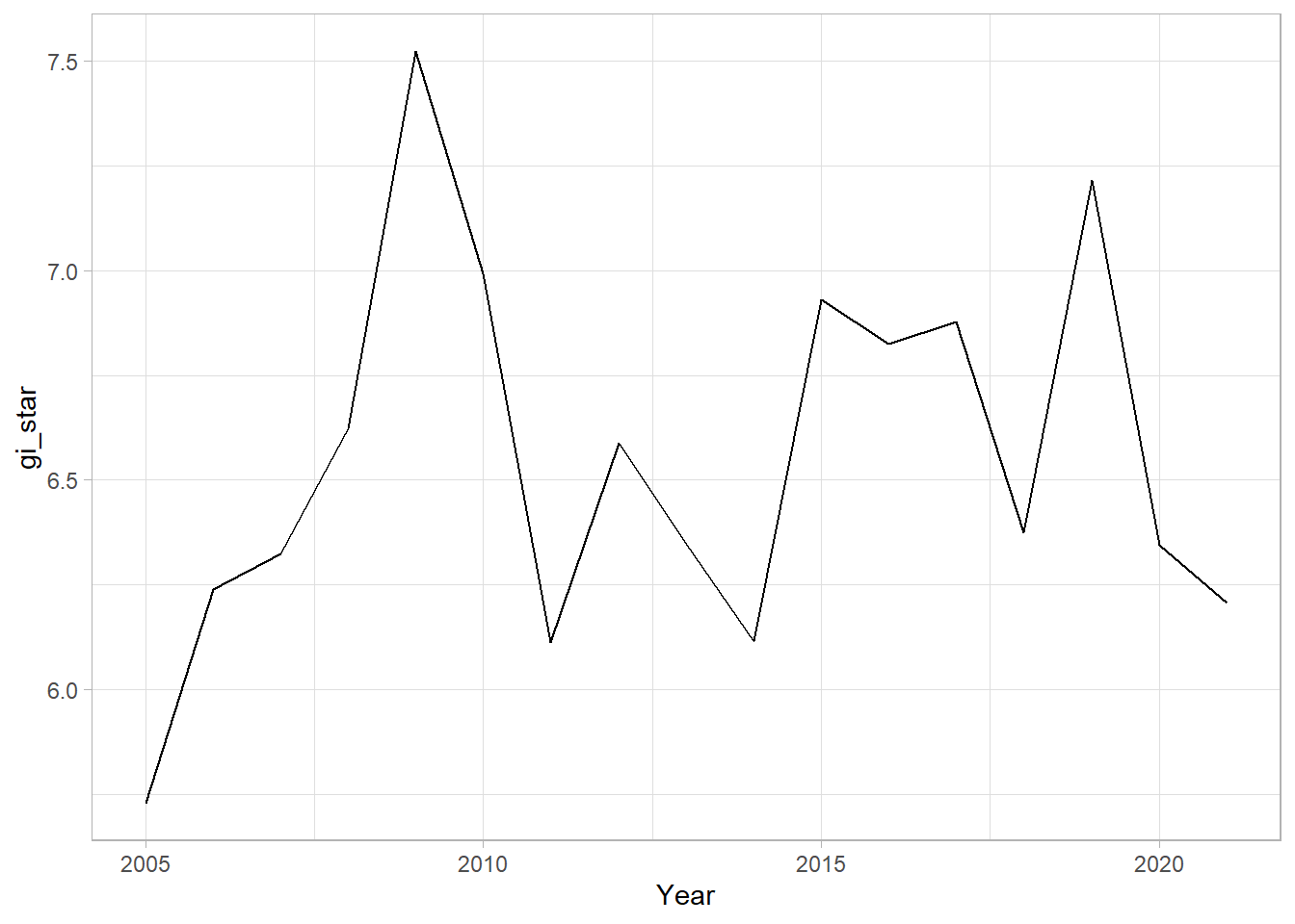

p <- ggplot(data = cbg, 
       aes(x = Year, 
           y = gi_star)) +
  geom_line() +
  theme_light()

ggplotly(p)

cbg %>%
  summarise(mk = list(
    unclass(
      Kendall::MannKendall(gi_star)))) %>% 
  tidyr::unnest_wider(mk)

# A tibble: 1 × 5
    tau    sl     S     D  varS
  <dbl> <dbl> <dbl> <dbl> <dbl>
1 0.132 0.484    18  136.  589.

ehsa <- gi_stars %>%
  group_by(County) %>%
  summarise(mk = list(
    unclass(
      Kendall::MannKendall(gi_star)))) %>%
  tidyr::unnest_wider(mk)

4.1 Arrange to Show Significant Emerging Hot/Cold Spots

emerging <- ehsa %>% 
  arrange(sl, abs(tau)) %>% 
  slice(1:5)

5 Performing Emerging Hotspot Analysis

ehsa <- emerging_hotspot_analysis(
  x = GDPPC_st, 
  .var = "GDPPC", 
  k = 1, 
  nsim = 99
)

5.1 Visualising the Distribution of EHSA Classes

ggplot(data = ehsa,
       aes(x = classification)) +
  geom_bar()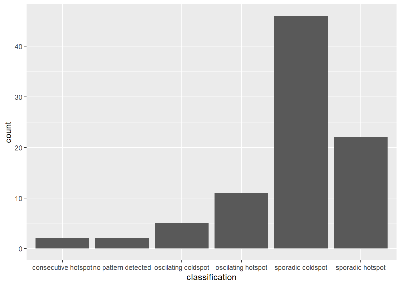

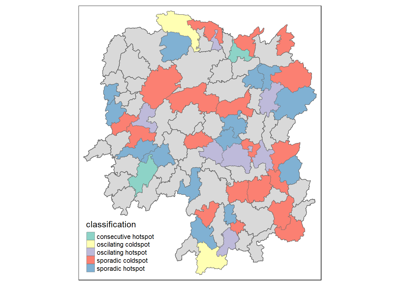
5.2 Visualising EHSA

hunan_ehsa <- hunan %>%
  left_join(ehsa,
           by =  c("County" = "location"))

ehsa_sig <- hunan_ehsa  %>%
  filter(p_value < 0.05)
tmap_mode("plot")
tm_shape(hunan_ehsa) +
  tm_polygons() +
  tm_borders(alpha = 0.5) +
tm_shape(ehsa_sig) +
  tm_fill("classification") + 
  tm_borders(alpha = 0.4)